Main Content

step

System object: phased.WidebandRadiator
Namespace: phased

Radiate wideband signals

Description

Note

Starting in R2016b, instead of using the step method to perform the operation defined by the System object™, you can call the object with arguments, as if it were a function. For example, y = step(obj,x) and y = obj(x) perform equivalent operations.

sigrad = step(sWBR,sig,ang) radiates the signal sig in the directions specified by ang. For each direction, the method computes the radiated signal, sigrad, by summing the contributions of each element or subarray.

example

sigrad = step(sWBR,sig,ang,laxes) radiates the signal using the specified the local coordinate system of the radiator, laxes. This syntax applies when you set the EnablePolarization property to true.

example

sigrad = step(sWBR,sig,ang,wts) radiates the signal using wts as the weight vector when the WeightsInputPort property is true.

sigrad = step(sWBR,sig,ang,steerang) radiates the signal and uses steerang as the subarray steering angle. steerang must be a length-2 column vector in the form of [AzimuthAngle; ElevationAngle]. This syntax applies when you use a subarray as the Sensor property and set the SubarraySteering property of the sensor to 'Phase' or 'Time'.

You can combine optional input arguments when you set their enabling properties in the System object during construction. Optional inputs must be listed in the same order as their enabling properties. For example, sigrad = step(sWBR,sig,laxes,wts,steerang) is valid when you set both EnablePolarization and WeightsInputPort to true and set the SubarraySteering property of the sensor.

Note

The object performs an initialization the first time the object is executed. This initialization locks nontunable properties and input specifications, such as dimensions, complexity, and data type of the input data. If you change a nontunable property or an input specification, the System object issues an error. To change nontunable properties or inputs, you must first call the release method to unlock the object.

Input Arguments

expand all

Wideband radiator, specified as a phased.WidebandRadiator System object.

Example: phased.WidebandRadiator

Input signals, specified as an M-by-1 complex-valued column vector or M-by-N complex-valued matrix. The quantity M is the number of sample values (snapshots) of the signal. If sig is a column vector, the same signal is radiated through all elements. If sig is a matrix, N is the number of sensor elements in the array. For subarrays, N is the number of subarrays. Each column of sig represents the field radiated by the corresponding element or subarray.

The size of the first dimension of the input matrix can vary to simulate a changing signal length. A size change can occur, for example, in the case of a pulse waveform with variable pulse repetition frequency.

Example: [[0;1;2;3;4;3;2;1;0],[1;2;3;4;3;2;1;0;0]]

Data Types: double
Complex Number Support: Yes

Radiating directions of the signal, specified as 2-by-L real-valued matrix or 1-by-L real-valued row vector. The quantity L is the number of directions to radiate. If ang is a matrix, each column has the form [azimuth;elevation]. If ang is a row vector, each entry represents the azimuthal direction. The elevation direction is zero degrees. Angle units are in degrees. Angles are defined with respect to the local coordinate system of the array.

When the sensory array is a uniform linear array, ang represents the broadside angle.

Data Types: double

Local coordinate system axes, specified as a 3-by-3 real-valued matrix orthonormal matrix. The matrix columns specify the x, y, and z axes of the local coordinate system. Each column takes the form [x;y;z] with respect to the global coordinate system. This argument only applies when the EnablePolarization property is set to true.

Data Types: double

Weight vector, specified as an N-by-1 complex-valued column vector. Each weight vector element multiplies the signal at the corresponding element or subarray. N is the number of radiating elements or subarrays. This argument only applies when the WeightsInputPort property is true.

Data Types: double
Complex Number Support: Yes

Subarray steering angle, specified as a 2-by-1 real-valued column vector in the form of [AzimuthAngle; ElevationAngle]. This argument applies only when the Sensor property refers to a subarray and the SubarraySteering property of the sensor is set to 'Phased' or 'Time'. Angles are defined with respect to the local coordinate system axes. Angle units are in degrees.

Data Types: double

Output Arguments

expand all

Radiated signal, returned as an M-by-L complex-valued matrix or 1-by-L array of struct type depending on whether polarization is enabled. The radiated field is the combined far-field output from all elements or subarrays. The quantity M is the number of sample values (snapshots) of the signal. The quantity L is the number of entries in ang.

  • If you set EnablePolarization to false, sigrad is an M-by-L complex-valued matrix.

  • If you set EnablePolarization is true, sigrad is a 1-by-L array of struct type. Each struct in the array has three data fields: sigrad.X, sigrad.Y, sigrad.Z which correspond to the x, y, and z components of the electromagnetic field. Electromagnetic field components are defined with respect to the global coordinate system. Each data field is an M-by-1 column vector.

Examples

expand all

Create a 5-by-5 URA and space the elements one-half wavelength apart. The wavelength corresponds to a design frequency of 300 MHz.

Create 5-by-5 URA Array of Cosine Elements

c = physconst('LightSpeed');
fc = 100e6;
lam = c/fc;
antenna = phased.CosineAntennaElement('CosinePower',[2,2]);
array = phased.URA('Element',antenna,'Size',[5,5],'ElementSpacing',[0.5,0.5]*lam);

Create and Radiate Wideband Signal

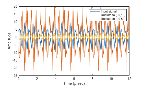
Radiate a wideband signal consisting of three sinusoids at 2, 10 and 11 MHz. Set the sampling rate to 25 MHz. Radiate the fields into two directions: (30,10) degrees azimuth and elevation and (20,50) degrees azimuth and elevation.

fs = 25e6;
f1 = 2e6;
f2 = 10e6;
f3 = 11e6;
dt = 1/fs;
Tsig = 100e-6;
t = [0:dt:Tsig];
sig = 5.0*sin(2*pi*f1*t) + 2.0*sin(2*pi*f2*t + pi/10) + 4*sin(2*pi*f3*t + pi/2); 
radiatingangles = [30 10; 20 50]';
radiator = phased.WidebandRadiator('Sensor',array,'CarrierFrequency',fc,'SampleRate',fs);
radsig = radiator(sig.',radiatingangles);

Plot Radiated Signal

Plot the input signal to the radiator and the radiated signals.

plot(t(1:300)*1e6,real(sig(1:300)))
hold on
plot(t(1:300)*1e6,real(radsig(1:300,1)))
plot(t(1:300)*1e6,real(radsig(1:300,2)))
hold off
xlabel('Time (\mu sec)')
ylabel('Amplitude')
legend('Input signal','Radiate to (30,10)','Radiate to (20,50)')

Figure contains an axes object. The axes object with xlabel Time ( mu sec), ylabel Amplitude contains 3 objects of type line. These objects represent Input signal, Radiate to (30,10), Radiate to (20,50).

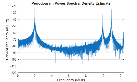
Plot the spectra of the signal that is radiated to (30,10) degrees.

periodogram(real(radsig(:,1)),rectwin(size(radsig,1)),4096,fs);

Figure contains an axes object. The axes object with title Periodogram Power Spectral Density Estimate, xlabel Frequency (MHz), ylabel Power/frequency (dB/Hz) contains an object of type line.

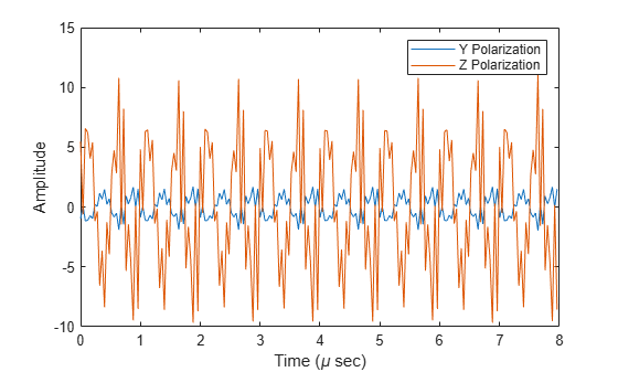
Examine the polarized field produced by the wideband radiator from a five-element uniform line array (ULA) composed of short-dipole antenna elements.

Set up the ULA of five short-dipole antennas with polarization enabled. The element spacing is set to 1/2 wavelength of the carrier frequency. Construct the wideband radiator System object™.

fc = 100e6;
c = physconst('LightSpeed');
lam = c/fc;
antenna = phased.ShortDipoleAntennaElement;
array = phased.ULA('Element',antenna,'NumElements',5,'ElementSpacing',lam/2);

Radiate a signal consisting of the sum of three sine waves. Radiate the signal into two different directions. Radiated angles are azimuth and elevation angles defined with respect to a local coordinate system. The local coordinate system is defined by 10 degree rotation around the x-axis from the global coordinates.

fs = 25e6;
f1 = 2e6;
f2 = 10e6;
f3 = 11e6;
dt = 1/fs;
fc = 100e6;
t = [0:dt:100e-6];
sig = 5.0*sin(2*pi*f1*t) + 2.0*sin(2*pi*f2*t + pi/10) + 4*sin(2*pi*f3*t + pi/2);
radiatingAngle = [30 30; 0 20];
laxes = rotx(10);
radiator = phased.WidebandRadiator('Sensor',array,'SampleRate',fs,...
    'CarrierFrequency',fc,'Polarization','Combined');
y = radiator(sig.',radiatingAngle,laxes);

Plot the first 200 samples of the y and z components of the polarized field propagating in the [30,0] direction.

plot(10^6*t(1:200),real(y(1).Y(1:200)))
hold on
plot(10^6*t(1:200),real(y(1).Z(1:200)))
hold off
xlabel('Time (\mu sec)')
ylabel('Amplitude')
legend('Y Polarization','Z Polarization')

Figure contains an axes object. The axes object with xlabel Time ( mu sec), ylabel Amplitude contains 2 objects of type line. These objects represent Y Polarization, Z Polarization.

Version History

Introduced in R2015b