Industrial Process Anomaly Detection using Statistical Process Control

This example demonstrates how Statistical Process Control (SPC) can be used for multivariate anomaly detection in a complex industrial process. Using simulated Tennessee Eastman Process (TEP) data, the example shows how to train, tune, and test an SPC-based detector to identify process anomalies caused by different fault types.

In this example, an anomaly is defined as a time window in which one or more monitored signals violate the SPC control limits. A fault refers to an underlying process condition (fault numbers 1–20) that may produce sustained or intermittent anomalies.

The typical workflow to train an SPC detector is as follows:

1. Select process signals that are stationary (stable) under normal operating conditions.

2. Train the detector with the selected signals.

3. Validate the detector with data that contains faults.

4. Adjust detector settings and go back to Step 2 as needed.

5. Test the detector with both normal and faulty test data.

Download Data Set

This example uses files formatted for MATLAB®. They were converted by MathWorks® from the Tennessee Eastman Process (TEP) simulation data [1]. These files are available at the MathWorks support files site. See the disclaimer.

The data set consists of four components: fault-free training, fault-free testing, faulty training, and faulty testing. Download each file separately.

url = "https://www.mathworks.com/supportfiles/predmaint/chemical-process-fault-detection-data/";
files = ["faultfreetraining.mat","faultfreetesting.mat","faultytraining.mat","faultytesting.mat"];
for f = files
    websave(f,url+f);
end

Load the downloaded files into the MATLAB workspace.

load('faultfreetraining.mat');
load('faultfreetesting.mat');
load('faultytraining.mat');
load('faultytesting.mat');

Each component contains data from simulations that were run for every permutation of two parameters: Fault Number and Simulation Run. The length of each simulation was dependent on the data set. All simulation data was sampled every 3 minutes.

• Training data sets contain 500 time samples from 25 hours of simulation.

• Testing data sets contain 960 time samples from 48 hours of simulation.

Each data table has the following variables in its columns:

• Column 1 (faultNumber) indicates the fault type, which varies from 0 through 20. A fault number 0 means fault-free while fault numbers 1 to 20 represent different fault types in the TEP process.

• Column 2 (simulationRun) indicates the simulation number of the TEP process. In the training and test data sets, the number of runs varies from 1 to 500 for all fault numbers. Every simulationRun value represents a different random number generator state used for the simulation.

• Column 3 (sample) indicates the times at which the TEP variables were recorded per simulation. The number varies from 1 to 500 for the training data sets and from 1 to 960 for the testing data sets. The TEP variables (columns 4 to 55) were sampled every 3 minutes for a duration of 25 hours and 48 hours for the training and testing data sets, respectively.

• Columns 4–44 (xmeas_1 through xmeas_41) contain the measured variables of the TEP.

• Columns 45–55 (xmv_1 through xmv_11) contain the manipulated variables of the TEP.

Examine part of the data.

head(faultfreetraining,5)

    faultNumber    simulationRun    sample    xmeas_1    xmeas_2    xmeas_3    xmeas_4    xmeas_5    xmeas_6    xmeas_7    xmeas_8    xmeas_9    xmeas_10    xmeas_11    xmeas_12    xmeas_13    xmeas_14    xmeas_15    xmeas_16    xmeas_17    xmeas_18    xmeas_19    xmeas_20    xmeas_21    xmeas_22    xmeas_23    xmeas_24    xmeas_25    xmeas_26    xmeas_27    xmeas_28    xmeas_29    xmeas_30    xmeas_31    xmeas_32    xmeas_33    xmeas_34    xmeas_35    xmeas_36    xmeas_37    xmeas_38    xmeas_39    xmeas_40    xmeas_41    xmv_1     xmv_2     xmv_3     xmv_4     xmv_5     xmv_6     xmv_7     xmv_8     xmv_9     xmv_10    xmv_11
    ___________    _____________    ______    _______    _______    _______    _______    _______    _______    _______    _______    _______    ________    ________    ________    ________    ________    ________    ________    ________    ________    ________    ________    ________    ________    ________    ________    ________    ________    ________    ________    ________    ________    ________    ________    ________    ________    ________    ________    ________    ________    ________    ________    ________    ______    ______    ______    ______    ______    ______    ______    ______    ______    ______    ______

         0               1            1       0.25038      3674       4529      9.232     26.889     42.402     2704.3     74.863     120.41     0.33818      80.044      51.435      2632.9      25.029      50.528      3101.1      22.819      65.732      229.61      341.22       94.64      77.047      32.188      8.8933      26.383       6.882      18.776      1.6567      32.958      13.823      23.978      1.2565      18.579      2.2633      4.8436      2.2986     0.017866     0.8357     0.098577     53.724      43.828     62.881    53.744    24.657    62.544    22.137    39.935    42.323    47.757     47.51    41.258    18.447
         0               1            2       0.25109    3659.4     4556.6     9.4264     26.721     42.576       2705         75     120.41      0.3362      80.078      50.154      2633.8      24.419      48.772        3102      23.333      65.716      230.54       341.3      94.595      77.434      32.188      8.8933      26.383       6.882      18.776      1.6567      32.958      13.823      23.978      1.2565      18.579      2.2633      4.8436      2.2986     0.017866     0.8357     0.098577     53.724      43.828     63.132    53.414    24.588    59.259    22.084    40.176    38.554    43.692    47.427    41.359    17.194
         0               1            3       0.25038    3660.3     4477.8     9.4426     26.875      42.07     2706.2     74.771     120.42     0.33563       80.22      50.302      2635.5      25.244      50.071      3103.5      21.924      65.732      230.08      341.38      94.605      77.466      31.767      8.7694      26.095      6.8259      18.961      1.6292      32.985      13.742      23.897      1.3001      18.765      2.2602      4.8543        2.39     0.017866     0.8357     0.098577     53.724      43.828     63.117    54.357    24.666    61.275     22.38    40.244     38.99    46.699    47.468    41.199     20.53
         0               1            4       0.24977    3661.3     4512.1     9.4776     26.758     42.063     2707.2     75.224     120.39     0.33553      80.305       49.99      2635.6      23.268      50.435      3102.8      22.948      65.781      227.91      341.71      94.473      77.443      31.767      8.7694      26.095      6.8259      18.961      1.6292      32.985      13.742      23.897      1.3001      18.765      2.2602      4.8543        2.39     0.017866     0.8357     0.098577     53.724      43.828       63.1    53.946    24.725    59.856    22.277    40.257    38.072    47.541    47.658    41.643    18.089
         0               1            5       0.29405      3679       4497     9.3381     26.889      42.65     2705.1     75.388     120.39     0.32632      80.064       51.31      2632.4      26.099       50.48      3103.5      22.808      65.788      231.37      341.11      94.678      76.947      32.322      8.5821      26.769      6.8688      18.782      1.6396      33.071      13.834      24.228      1.0938      18.666      2.2193      4.8304      2.2416     0.017866     0.8357     0.098577     53.724      43.828     63.313    53.658    28.797    60.717    21.947    39.144    41.955    47.645    47.346    41.507    18.461

Select Stationary Data Channels

Anomaly detection using Statistical Process Control techniques relies on finding process signals that are stationary (stable) under normal operating conditions of the process. In this example, stationarity is assessed through visual inspection of fault-free signal channels. Additional preprocessing such as detrending, seasonal decomposition, or normalization may be required prior to SPC modeling.

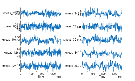
With visual inspection of fault-free training data, select a number of stationary data channels for training and testing the detector. These channels exhibit relatively stable behavior under normal operating conditions and are known to be sensitive to multiple TEP fault types.

As an example, visualize the selected signals for simulation 35. The helper function helperExtract is used to extract selected parts of data from training and testing data sets for a given simulation number and a fault type.

channels = [...
    "xmeas_2","xmeas_6","xmeas_10","xmeas_12","xmeas_22",...
    "xmeas_24","xmeas_28","xmeas_30","xmeas_34","xmeas_36"];

simulationRun = 35;

data = helperExtract(0,simulationRun,channels,"training");

figure;
tiledlayout(1,2)
nexttile
stackedplot(data(:,1:5));
nexttile
stackedplot(data(:,6:end));

Train the SPC Detector

Fault-free training data set has all 500 simulations of the industrial process in a single table. Extract each simulation as an element of a cell array of timetables, which is one of the data formats recognized by the SPC anomaly detector.

N = 500;
trainingData = cell(N,1);
for n = 1:N
    trainingData{n} = helperExtract(0,n,channels,"training");
end

Train the anomaly detector using all 500 fault-free simulations. The detector settings can be assigned using an analysis procedure with the following considerations:

• Batch the data to minimize the number of data points used for anomaly detection and reduce the autocorrelation of the signals when the sampling rate is faster than the normal system dynamics of the TEP process. Set the WindowLength to 10 to reduce the 500 samples to an averaged set of 50 samples.

• Capture the variation of data under normal operating conditions to minimize the number of false positives when evaluating the trained detector against the training data. Set Level to 5 to treat the variation of signals as normal when they stay within 5 standard deviations of their mean.

• Detect anomalies only when the data wanders outside the upper and lower control limits of the SPC model. Set DetectionRules to empty to stop imposing additional anomaly detection rules on the model. See controlrules for further details of this setting.

• Use the Exponentially-Weighted Moving Average method with a smaller smoothing factor to take the history of the signals into account for anomaly detection. Set Method to "ewma" and the smoothing parameter Lambda to 0.2.

numChannels = numel(channels);
h = timeSeriesSpcAD(numChannels,WindowLength=10,Level=5.0,DetectionRules=[]);
h = train(h,trainingData,Method="ewma",Lambda=0.2);

The detector trains the model using various statistical measures of all signals from the entire fault-free training data set. These statistics are used to compute the upper and lower control limits (UCL and LCL) for anomaly detection.

h

h = 
  TimeSeriesSPCDetector with properties:

       NumChannels: 10
      WindowLength: 10
            Stride: 10
            Method: "ewma"
            Lambda: 0.2000
    DetectionRules: [1×0 string]
             Level: 5
        CenterLine: [3.6638e+03 42.3376 0.3371 49.9996 77.2948 8.8935 1.6568 13.8228 2.2633 2.2983]
     StandardError: [4.8962 0.0251 0.0025 0.1067 0.0340 0.0175 0.0042 0.0200 0.0047 0.0090]
              Mean: [3.6638e+03 42.3376 0.3371 49.9996 77.2948 8.8935 1.6568 13.8228 2.2633 2.2983]
             Sigma: [14.6886 0.0752 0.0074 0.3200 0.1021 0.0525 0.0126 0.0599 0.0142 0.0271]
         MeanRange: [16.8320 0.0812 0.0064 0.3617 0.0808 0.0528 0.0129 0.0567 0.0132 0.0266]
         IsTrained: 1

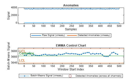
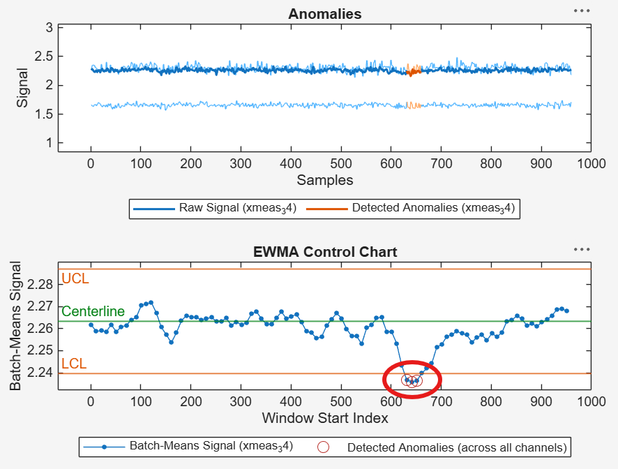
The trained model should ideally not detect any false anomalies in the fault-free training data. Visualize detection on simulation 35, where no anomalies are detected as expected. Note that the plot function includes a detection step when input data is provided.

figure;
plot(h,trainingData(simulationRun),"PlotType","anomaly")

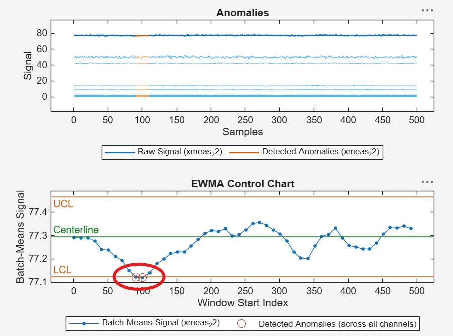
In the worst case, out of 500 fault-free simulations, only two data windows in simulation 42 were likely considered to be an anomaly, where the signal xmeas_22 slightly goes outside its lower control limit (LCL).

trainingResults = detect(h,trainingData);

numAnomalies = helperNumAnomalies(trainingResults);
[maxAnomalies,simIndex] = max(numAnomalies) %#ok<ASGLU>

maxAnomalies = 
2

simIndex = 
42

Visualize anomaly detection on simulation 42. Run the following code in the Command Window for an interactive view of the two detected anomalies in simulation 42.

plot(h,trainingData(simIndex),"PlotType","anomaly");

As an alternative, the Level parameter of the detector can be further increased to fully eliminate these edge cases, for example, by running the following code in the Command Window before retraining the detector:

h = updateDetector(h,[],"Level",5.5);

Considering the possibility of probabilistic occurrence of anomalies when using SPC techniques, set a small health threshold to separate normal signals from anomalous signals. The health threshold indicates the maximum number of detected anomalies that can be tolerated as random occurrences in a healthy process.

Set the health threshold to 2, which results in no false positives and all true negatives (that is, no anomalies detected) as would be expected when using the fault-free training data.

healthyThreshold = 2;

trueLabels = categorical(false(500,1),[true,false],{'Anomaly','No Anomaly'});
predictedLabels = categorical(numAnomalies>healthyThreshold,[true,false],{'Anomaly','No Anomaly'});

figure;
confusionchart(trueLabels,predictedLabels,ZerosVisible=true);
title('Anomaly Detection on Fault-Free Training Data');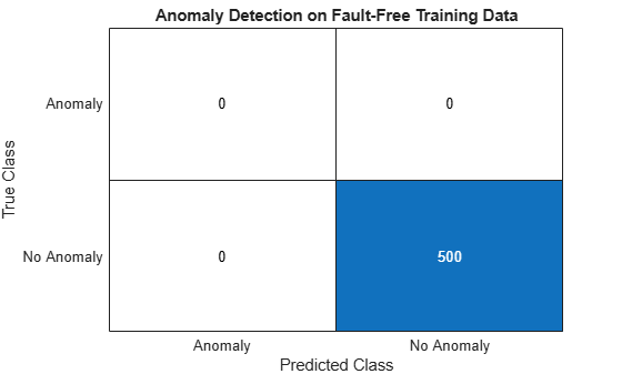

The detector performs perfectly on normal training data with no false positives.

Evaluate the Trained SPC Detector

Evaluate the performance of the trained detector for identifying which candidate fault types could be detected most successfully. Compile an evaluation data set consisting of a single simulation per each fault type.

N = 20;
evaluationData = cell(N,1);
for n = 1:N
    evaluationData{n} = helperExtract(n,simulationRun,channels,"training");
end

The trained detector using the selected signal channels is able to detect anomalies in simulations involving different fault types. Investigate which fault types are most likely to be detected successfully using the faulty training data set for simulation 35.

evaluationResults = detect(h,evaluationData);
numAnomalies = helperNumAnomalies(evaluationResults);

The detector identifies anomalies in simulations involving various fault types. Using the selected signal channels, the fault type 2 is most readily identified with most number of detected anomalies. Similarly, the anomalies in signals with fault types 1, 6, 8, 12, 13, and 18 are also detected with high confidence (more than 40 anomalous data windows out of 50 batch-means windowed samples).

candidateFaults = find(numAnomalies>healthyThreshold)'

candidateFaults = 1×10

    1    2    5    6    7    8    12    13    18    20

numDetectedAnomalies = numAnomalies(candidateFaults)'

numDetectedAnomalies = 1×10

    45    47    13    44    16    41    44    43    45    22

Set a fault threshold of 20 to ensure satisfactory detector performance before testing the trained detector against all simulations for the selected fault type. The fault threshold indicates the minimum number of anomalous windows required to classify a simulation as faulty.

faultyThreshold = 20;

[~,faultNumber] = max(numAnomalies)

faultNumber = 
2

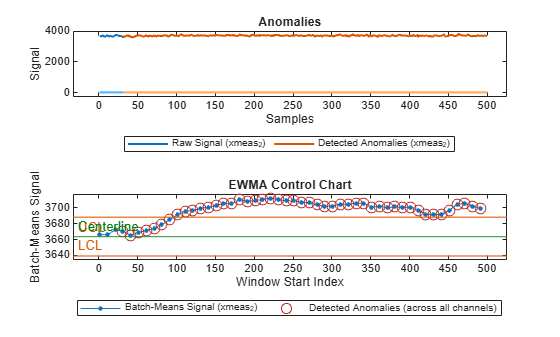
Visualize fault detection on simulation 35 for fault type 2. Notice that most data points are detected as anomalies because they fall outside the upper control limits (UCL) in at least one of the signal channels used for detection.

figure;
plot(h,evaluationData(faultNumber),"PlotType","anomaly");

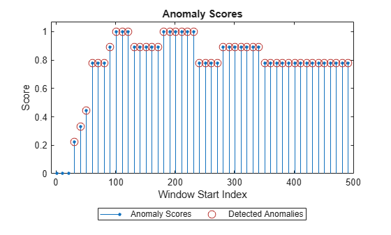
Visualize the corresponding anomaly scores, indicating high confidence in anomaly detection when one or more signals move outside their control limits.

figure;
plot(h,evaluationData(faultNumber),"PlotType","anomalyScores");

The same trained detector can be used to detect anomalies in simulations involving one or more of the candidate fault types identified above. Proceed with only the selected fault type (fault number 2) for simplicity.

Validate the Trained SPC Detector

Now, validate the trained detector against all 500 training simulations of the selected fault type (fault number 2).

N = 500;
validationData = cell(N,1);
for n = 1:N
    validationData{n} = helperExtract(faultNumber,n,channels,"training");
end

Visualize the selected signals for simulation 35 of the selected fault type. Notice that most of the signals no longer exhibit a stationary behavior when the fault is present in the TEP process.

data = validationData{simulationRun};

figure;
tiledlayout(1,2)
nexttile
stackedplot(data(:,1:5));
nexttile
stackedplot(data(:,6:end));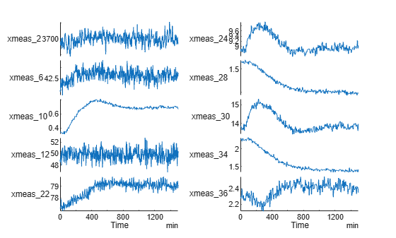

The trained detector using the selected signal channels is able to detect anomalies in all simulations involving the selected fault type.

validationResults = detect(h,validationData);
numAnomalies = helperNumAnomalies(validationResults);

In all simulations with fault type 2, the detector is able to identify a large number of anomalous data windows in the signals.

[minAnomalies,simIndex] = min(numAnomalies) %#ok<ASGLU>

minAnomalies = 
46

simIndex = 
9

Visualize fault detection for the worst case (that is, least number of detected anomalies). Notice that, even in this least successful case, most data windows are detected as anomalies because they fall outside the control limits for at least one of the signal channels used for detection.

figure;
plot(h,validationData(simIndex),"PlotType","anomaly")

Setting the fault threshold to 20 resulted in all true positives (that is, all anomalies detected) and no false negatives as would be expected when using the faulty training data set.

trueLabels = categorical(true(500,1),[true,false],{'Anomaly','No Anomaly'});
predictedLabels = categorical(numAnomalies>faultyThreshold,[true,false], {'Anomaly','No Anomaly'});

figure;
confusionchart(trueLabels,predictedLabels,ZerosVisible=true);
title('Anomaly Detection on Faulty Training Data for Fault Number 2');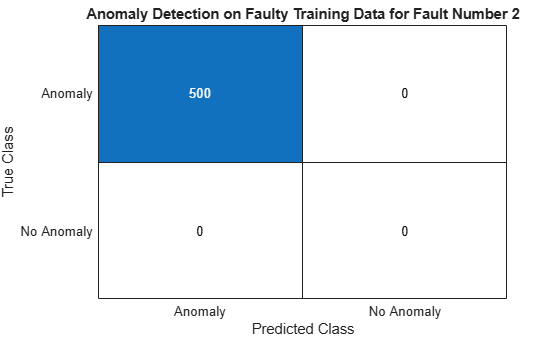

The detector performs perfectly on faulty training data with no false negatives when fault type 2 is present in the process.

Test against all Simulations of Fault-Free Process

Once the training and validation of the SPC detector is complete, test the performance of the detector on independent test data set for fault-free and faulty simulations of the TEP process.

Start testing the model with fault-free simulation data to identify false positives, if any.

N = 500;
testFaultFreeData = cell(N,1);
for n = 1:N
    testFaultFreeData{n} = helperExtract(0,n,channels,"testing");
end

Run the SPC detector on the data set.

testFaultFreeResults = detect(h,testFaultFreeData);
numAnomalies = helperNumAnomalies(testFaultFreeResults);

The detector flags only one simulation of the fault-free system (out of 500) as a potential anomaly.

[maxAnomalies,simIndex] = max(numAnomalies) %#ok<ASGLU>

maxAnomalies = 
3

simIndex = 
240

Visualize anomaly detection on simulation 240 to analyze the reason for the false positive identification. Run the following code in the Command Window for an interactive view of the detected anomalies for simulation 240.

plot(h,testFaultFreeData(simIndex),"PlotType","anomaly")

Only three data points for simulation 240 were likely considered to be an anomaly, where the signal xmeas_34 slightly goes outside its lower control limit (LCL).

Using the fault-free testing data, the detector identifies only a single false positive (that is, an anomaly when there is in fact none) out of 500 simulations.

trueLabels = categorical(false(500,1),[true,false],{'Anomaly','No Anomaly'});
predictedLabels = categorical(numAnomalies>healthyThreshold,[true,false],{'Anomaly','No Anomaly'});

figure;
confusionchart(trueLabels, predictedLabels, ZerosVisible=true);
title('Anomaly Detection on Fault-Free Testing Data');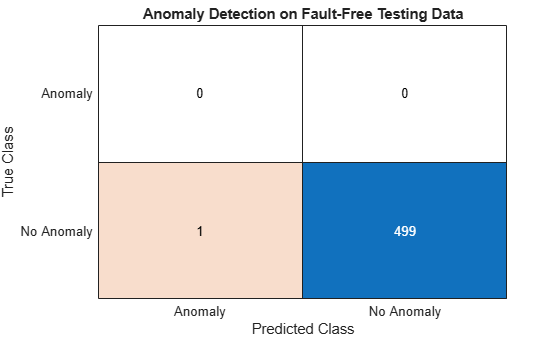

The detector performs well on fault-free testing data with an acceptable false positive rate (1 out of 500).

Test against all Simulations of Faulty Process

Continue testing the SPC detector with simulation data for faulty cases to identify false negatives, if any.

N = 500;
testFaultyData = cell(N,1);
for n = 1:N
    testFaultyData{n} = helperExtract(faultNumber,n,channels,"testing");
end

Run the SPC detector on the data set.

testFaultyResults = detect(h,testFaultyData);
numAnomalies = helperNumAnomalies(testFaultyResults);

The detector flags all simulations as containing anomalies as expected in this testing scenario. Notice that, even in the least successful case, most data windows are detected as anomalies because they fall outside the control limits for at least one of the signal channels used for detection.

[minAnomalies,simIndex] = min(numAnomalies)

minAnomalies = 
78

simIndex = 
1

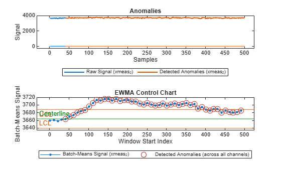
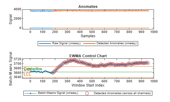
Visualize anomaly detection on simulation 1. Notice that anomalies are detected consistently across multiple channels once the fault is introduced, indicating strong sensitivity of the SPC detector to this fault type.

figure;
plot(h,testFaultyData(simIndex),"PlotType","anomaly")

Visualize the corresponding anomaly scores, indicating high confidence in anomaly detection when one or more signals move outside their control limits.

figure;
plot(h,testFaultyData(simIndex),"PlotType","anomalyScores");

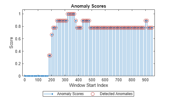
Using the faulty testing data for fault type 2, the detector identifies no false negative (that is, no anomaly when there is in fact one).

trueLabels = categorical(true(500,1),[true,false],{'Anomaly','No Anomaly'});
predictedLabels = categorical(numAnomalies>faultyThreshold,[true,false],{'Anomaly','No Anomaly'});

figure;
confusionchart(trueLabels,predictedLabels,ZerosVisible=true);
title('Anomaly Detection on Faulty Testing Data for Fault Number 2');

The detector performs perfectly on testing data with no false negatives when fault type 2 is present in the process.

Conclusion

Given a selection of suitable signals, the SPC-based anomaly detector can be trained to detect anomalies in the industrial process due to one or more fault types occurring in the system. After a simple selection of multiple data channels, the trained SPC detector performed well on the test data, generating no false negatives and only a single false positive out of 500 test simulations for the selected fault type. The SPC method is well suited as a baseline or early-warning layer in industrial monitoring systems.

References

[1] Rieth, Cory A.; Amsel, Ben D.; Tran, Randy; Cook, Maia B., 2017, "Additional Tennessee Eastman Process Simulation Data for Anomaly Detection Evaluation", https://doi.org/10.7910/DVN/6C3JR1, Harvard Dataverse, V1.

Helper Functions

helperExtract

The helper function helperExtract is used to extract training and testing data from the TEP database for any combination of a simulation run and a fault type. The data channels of interest (measured and manipulated variables) can also be specified by name. The result is returned as a timetable with sampling rate set to 3 minutes.

function T = helperExtract(faultNumber,simulationRun,dataChannels,dataType)
    arguments
        faultNumber (1,1) double {mustBeGreaterThanOrEqual(faultNumber,0),mustBeLessThanOrEqual(faultNumber,20)}
        simulationRun (1,1) double {mustBeGreaterThanOrEqual(simulationRun,1),mustBeLessThanOrEqual(simulationRun,500)}
        dataChannels (1,:) string
        dataType (1,1) string {mustBeMember(dataType,["training","testing"])}
    end

    switch dataType
        case "training"
            healthyVar = "faultfreetraining";
            faultyVar  = "faultytraining";
        case "testing"
            healthyVar = "faultfreetesting";
            faultyVar  = "faultytesting";
    end

    if faultNumber == 0
        baseVar = healthyVar;
    else
        baseVar = faultyVar;
    end

    T = evalin('base',baseVar);
    T = T((T.simulationRun==simulationRun)&(T.faultNumber==faultNumber),dataChannels);
    T = table2timetable(T,"TimeStep",minutes(3));
end

helperNumAnomalies

The helper function helperNumAnomalies is used to extract the number of anomalies from anomaly detection results for given industrial process simulations.

function numAnomalies = helperNumAnomalies(detectionResults)
    numAnomalies = cellfun(@(c)sum(c.Labels==true),detectionResults);
end