step

Simulate clutter using constant gamma model

Since R2021a

Starting in R2016b, instead of using the step method to perform the operation defined by the System object™, you can call the object with arguments, as if it were a function. For example, y = step(obj,x) and y = obj(x) perform equivalent operations.

Syntax

Y = step(H)

Y = step(H,X)

Y = step(H,STEERANGLE)

Y = step(H,X,WS)

Y = step(H,PRFIDX)

Y = step(H,X,STEERANGLE)

Description

Y = step(H) computes the collected clutter return at each sensor. This syntax is available when you set the TransmitSignalInputPort property to false.

Y = step(H,X) specifies the transmit signal in X. Transmit signal refers to the output of the transmitter while it is on during a given pulse. This syntax is available when you set the TransmitSignalInputPort property to true.

Y = step(H,STEERANGLE) uses STEERANGLE as the subarray steering angle. This syntax is available when you configure H so that H.Sensor is an array that contains subarrays and H.Sensor.SubarraySteering is either 'Phase' or 'Time'.

Y = step(H,X,WS) uses WS as weights applied to each element within each subarray. To use this syntax, set the Sensor property to an array that supports subarrays and set the SubarraySteering property of the array to 'Custom'.

Y = step(H,PRFIDX) uses the index, PRFIDX, to select the PRF from a predetermined list of PRFs specified by the PRF property. To enable this syntax, set the PRFSelectionInputPort to true.

Y = step(H,X,STEERANGLE) combines all input arguments. This syntax is available when you configure H so that H.TransmitSignalInputPort is true, H.Sensor is an array that contains subarrays, and H.Sensor.SubarraySteering is either 'Phase' or 'Time'.

Examples

Simulate Clutter for System with Known Power

Simulate the clutter return from terrain with a gamma value of 0 dB. The effective transmitted power of the radar system is 5 kW.

Set up the characteristics of the radar system. This system uses a four-element uniform linear array (ULA). The sample rate is 1 MHz, and the PRF is 10 kHz. The propagation speed is the speed of light, and the operating frequency is 300 MHz. The radar platform is flying 1 km above the ground with a path parallel to the ground along the array axis. The platform speed is 2 km/s. The mainlobe has a depression angle of 30°.

Nele = 4;
c = physconst('Lightspeed');
fc = 300.0e6;
lambda = c/fc;
array = phased.ULA('NumElements',Nele,'ElementSpacing',lambda/2);
fs = 1.0e6;
prf = 10.0e3;
height = 1000.0;
direction = [90;0];
speed = 2.0e3;
depang = 30.0;
mountingAng = [depang,0,0];

Create the clutter simulation object. The configuration assumes the earth is flat. The maximum clutter range of interest is 5 km, and the maximum azimuth coverage is ±60°.

Rmax = 5000.0;
Azcov = 120.0;
tergamma = 0.0;
tpower = 5000.0;
clutter = constantGammaClutter('Sensor',array,...
    'PropagationSpeed',c,'OperatingFrequency',fc,'PRF',prf,...
    'SampleRate',fs,'Gamma',tergamma,'EarthModel','Flat',...
    'TransmitERP',tpower,'PlatformHeight',height,...
    'PlatformSpeed',speed,'PlatformDirection',direction,...
    'MountingAngles',mountingAng,'ClutterMaxRange',Rmax,...
    'ClutterAzimuthSpan',Azcov,'SeedSource','Property',...
    'Seed',40547);

Simulate the clutter return for 10 pulses.

Nsamp = fs/prf;
Npulse = 10;
sig = zeros(Nsamp,Nele,Npulse);
for m = 1:Npulse
    sig(:,:,m) = clutter();
end

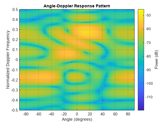
Plot the angle-Doppler response of the clutter at the 20th range bin.

response = phased.AngleDopplerResponse('SensorArray',array,...
    'OperatingFrequency',fc,'PropagationSpeed',c,'PRF',prf);
plotResponse(response,shiftdim(sig(20,:,:)),'NormalizeDoppler',true)

Simulate Clutter Using Known Transmit Signal

Simulate the clutter return from terrain with a gamma value of 0 dB. You input the transmit signal of the radar system when creating clutter. In this case, you do not use the TransmitERP property.

Set up the characteristics of the radar system. This system has a 4-element uniform linear array (ULA). The sample rate is 1 MHz, and the PRF is 10 kHz. The propagation speed is the speed of light, and the operating frequency is 300 MHz. The radar platform is flying 1 km above the ground with a path parallel to the ground along the array axis. The platform speed is 2 km/s. The mainlobe has a depression angle of 30°.

Nele = 4;
c = physconst('Lightspeed');
fc = 300.0e6;
lambda = c/fc;
ula = phased.ULA('NumElements',Nele,'ElementSpacing',lambda/2);
fs = 1.0e6;
prf = 10.0e3;
height = 1.0e3;
direction = [90;0];
speed = 2.0e3;
depang = 30;
mountingAng = [depang,0,0];

Create the clutter simulation object and configure it to accept an transmit signal as an input argument. The configuration assumes the earth is flat. The maximum clutter range of interest is 5 km, and the maximum azimuth coverage is ±60°.

Rmax = 5000.0;
Azcov = 120.0;
tergamma = 0.0;
clutter = constantGammaClutter('Sensor',ula,...
    'PropagationSpeed',c,'OperatingFrequency',fc,'PRF',prf,...
    'SampleRate',fs,'Gamma',tergamma,'EarthModel','Flat',...
    'TransmitSignalInputPort',true,'PlatformHeight',height,...
    'PlatformSpeed',speed,'PlatformDirection',direction,...
    'MountingAngles',mountingAng,'ClutterMaxRange',Rmax,...
    'ClutterAzimuthSpan',Azcov,'SeedSource','Property',...
    'Seed',40547);

Simulate the clutter return for 10 pulses. At each step, pass the transmit signal as an input argument. The software computes the effective transmitted power of the signal. The transmit signal is a rectangular waveform with a pulse width of 2 μs.

tpower = 5.0e3;
pw = 2.0e-6;
X = tpower*ones(floor(pw*fs),1);
Nsamp = fs/prf;
Npulse = 10;
sig = zeros(Nsamp,Nele,Npulse);
for m = 1:Npulse
    sig(:,:,m) = step(clutter,X);
end

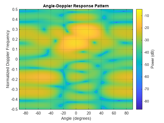
Plot the angle-Doppler response of the clutter at the 20th range bin.

response = phased.AngleDopplerResponse('SensorArray',ula,...
    'OperatingFrequency',fc,'PropagationSpeed',c,'PRF',prf);
plotResponse(response,shiftdim(sig(20,:,:)),'NormalizeDoppler',true)

Input Arguments

H — Constant gamma clutter object

constantGammaClutter System object

Constant gamma clutter object, specified as a constantGammaClutter System object.

X — Transmit signal

column vector

Transmit signal, specified as a column vector.

STEERANGLE — Subarray steering angle

length-2 column vector | scalar

Subarray steering angle in degrees, specified as a length-2 column vector or a scalar.

• If STEERANGLE is a length-2 vector, it has the form [azimuth; elevation]. The azimuth angle must be between –180 degrees and 180 degrees, and the elevation angle must be between –90 degrees and 90 degrees.

• If STEERANGLE is a scalar, it represents the azimuth angle. In this case, the elevation angle is assumed to be 0.

WS — Subarray element weights

matrix | cell array

Subarray element weights, specified as a complex-valued N_SE-by-N matrix or 1-by-N cell array, where N is the number of subarrays. These weights are applied to the individual elements within a subarray.

Subarray Element Weights

Sensor Array	Subarray Weights
phased.ReplicatedSubarray	All subarrays have the same dimensions and sizes. Then, the subarray weights form an NSE-by-N matrix. NSE is the number of elements in each subarray and N is the number of subarrays. Each column of WS specifies the weights for the corresponding subarray.
phased.PartitionedArray	When subarrays do not have the same dimensions and sizes, you can specify subarray weights as an NSE-by-N matrix, where NSE is now the number of elements in the largest subarray. The first Q entries in each column are the element weights for the subarray where Q is the number of elements in the subarray. a 1-by-N cell array. Each cell contains a column vector of weights for the corresponding subarray. The column vectors have lengths equal to the number of elements in the corresponding subarray.

Dependencies

To enable this argument, set the Sensor property to an array that contains subarrays and set the SubarraySteering property of the array to 'Custom'.

Complex Number Support: Yes

PRFIDX — Index of pulse repetition frequency

positive integer

Index of pulse repetition frequency, specified as a positive integer. The index selects one of the entries specified in the PRF property as the PRF for the next transmission.

Example: 3

Dependencies

To enable this argument, set the PRFSelectionInputPort to true.

Output Arguments

Y — Collected clutter return at each sensor

matrix

Collected clutter return at each sensor, returned as a matrix of dimensions N-by-M. If H.Sensor contains subarrays, M is the number of subarrays in the radar system. Otherwise it is the number of sensors. When you set the OutputFormat property to 'Samples', N is defined by the NumSamples property. When you set the OutputFormat property to 'Pulses', N is the total number of samples in the next L pulses. In this case, L is defined by the NumPulses property.

Tips

The clutter simulation that constantGammaClutter provides is based on these assumptions:

• The radar system is monostatic.

• The propagation is in free space.

• The terrain is homogeneous.

• The clutter patch is stationary during the coherence time. Coherence time indicates how frequently the software changes the set of random numbers in the clutter simulation.

• Because the signal is narrowband, the spatial response and Doppler shift can be approximated by phase shifts.

• The radar system maintains a constant height during simulation.

• The radar system maintains a constant speed during simulation.

Extended Capabilities

C/C++ Code Generation
Generate C and C++ code using MATLAB® Coder™.

Version History

Introduced in R2021a