Maritime Radar Sea Clutter Modeling
This example will introduce a sea clutter simulation for a maritime surveillance radar system. This example first discusses the physical properties associated with sea states. Next, it discusses the reflectivity of sea surfaces, investigating the effect of sea state, frequency, polarization, and grazing angle. Lastly, the example calculates the clutter-to-noise ratio (CNR) for a maritime surveillance radar system, considering the propagation path and weather effects.
Overview of Sea States
In describing sea clutter, it is important first to establish the physical properties of the sea surface. In modeling sea clutter for radar, there are three important parameters:
is the standard deviation of the wave height. The wave height is defined as the vertical distance between the wave crest and the adjacent wave trough.
is the slope of the wave.
is the wind speed.
Due to the irregularity of waves, the physical properties of the sea are often described in terms of sea states. The Douglas sea state number is a widely used scale that represents a wide range of physical sea properties such as wave heights and associated wind velocities. At the lower end of the scale, a sea state of 0 represents a calm, glassy sea state. The scale then proceeds from a slightly rippled sea state at 1 to rough seas with high wave heights at sea state 5. Wave heights at a sea state of 8 can be greater than 9 meters or more.
Using the searoughness function, plot the sea properties for sea states 1 through 5. Note the slow increase in the wave slope with sea state. This is a result of the wavelength and wave height increasing with wind speed, albeit with different factors.
% Analyze for sea states 1 through 5
ss = 1:5; % Sea states

% Initialize outputs
numSeaStates = numel(ss);
hgtsd = zeros(1,numSeaStates);
beta0 = zeros(1,numSeaStates);
vw= zeros(1,numSeaStates);

% Obtain sea state properties
for is = 1:numSeaStates
    [hgtsd(is),beta0(is),vw(is)] = searoughness(ss(is));
end

% Plot results
helperPlotSeaRoughness(ss,hgtsd,beta0,vw);
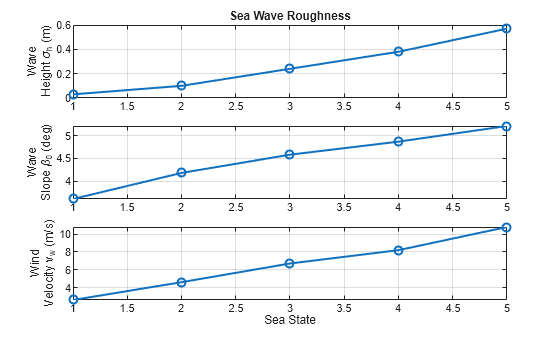
The physical properties you introduce is an important part in developing the geometry and environment of the maritime scenario. Furthermore, as you will see, radar returns from a sea surface exhibit strong dependence on sea state.
Reflectivity
The sea surface is composed of water with an average salinity of about 35 parts per thousand. The reflection coefficient of sea water is close to 1 for microwave frequencies and at low grazing angles.
For smooth seas, the wave height is small, and the sea appears as an infinite, flat conductive plate with little-to-no backscatter. As the sea state number increases and the wave height increases, the surface roughness increases. This results in increased scattering that is directionally dependent. Additionally, the reflectivity exhibits a strong proportional dependence on wave height and a dependence that increases with increasing frequency on wind speed.
Investigate sea surface reflectivity versus frequency for various sea states using the seareflectivity function. Set the grazing angle equal to 0.5 degrees and consider frequencies over the range of 500 MHz to 35 GHz.
grazAng = 0.5; % Grazing angle (deg)
freq = linspace(0.5e9,35e9,100); % Frequency (Hz)
pol = 'H'; % Horizontal polarization

% Initialize reflectivity output
numFreq = numel(freq);
nrcsH = zeros(numFreq,numSeaStates);

% Calculate reflectivity
for is = 1:numSeaStates
    nrcsH(:,is) = seareflectivity(ss(is),grazAng,freq,'Polarization',pol);
end

% Plot reflectivity
helperPlotSeaReflectivity(ss,grazAng,freq,nrcsH,pol);
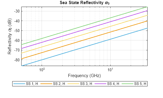
The figure shows that the sea surface reflectivity is proportional to frequency. Additionally, as the sea state number increases, which corresponds to increasing roughness, the reflectivity also increases.
Polarization Effects
Next, consider polarization effects on the sea surface reflectivity. Maintain the same grazing angle and frequency span from the previous section.
pol = 'V'; % Vertical polarization

% Initialize reflectivity output
numFreq = numel(freq);
nrcsV = zeros(numFreq,numSeaStates);

% Calculate reflectivity
for is = 1:numSeaStates
    nrcsV(:,is) = seareflectivity(ss(is),grazAng,freq,'Polarization',pol);
end

% Plot reflectivity
hAxes = helperPlotSeaReflectivity(ss,grazAng,freq,nrcsH,'H');
helperPlotSeaReflectivity(ss,grazAng,freq,nrcsV,'V',hAxes);

The figure shows that there is a noticeable effect on the reflectivity based on polarization. Notice that the difference between horizontal and vertical polarizations is greater at lower frequencies than at higher frequencies. As the sea state number increases, the difference between horizontal and vertical polarizations decreases. Thus, there is a decreasing dependence on polarization with increasing frequency.
Grazing Angle Effects
Consider the effect of grazing angle. Compute the sea reflectivity over the range of 0.1 to 60 degrees at an L-band frequency of 1.5 GHz.
grazAng = linspace(0.1,60,100); % Grazing angle (deg)
freq = 1.5e9; % L-band frequency (Hz)

% Initialize reflectivity output
numGrazAng = numel(grazAng);
nrcsH = zeros(numGrazAng,numSeaStates);
nrcsV = zeros(numGrazAng,numSeaStates);

% Calculate reflectivity
for is = 1:numSeaStates
    nrcsH(:,is) = seareflectivity(ss(is),grazAng,freq,'Polarization','H');
    nrcsV(:,is) = seareflectivity(ss(is),grazAng,freq,'Polarization','V');
end

% Plot reflectivity
hAxes = helperPlotSeaReflectivity(ss,grazAng,freq,nrcsH,'H');
helperPlotSeaReflectivity(ss,grazAng,freq,nrcsV,'V',hAxes);
ylim(hAxes,[-60 -10]);

From the figure, note that there is much more variation in the sea reflectivity at lower grazing angles, and differences exist between vertical and horizontal polarization. The figure shows that the dependence on grazing angle decreases as the grazing angle increases. Furthermore, the reflectivity for horizontally polarized signals is less than vertically polarized signals for the same sea state over the range of grazing angles considered.
Maritime Surveillance Radar Example
Calculating Clutter-to-Noise Ratio
Consider a horizontally polarized maritime surveillance radar system operating at 6 GHz (C-band). Define the radar system.
% Radar parameters
freq = 6e9;         % C-band frequency (Hz)
anht = 20;          % Height (m)
ppow = 200e3;       % Peak power (W)
tau  = 200e-6;      % Pulse width (sec)
prf  = 300;         % PRF (Hz)
azbw = 10;          % Half-power azimuth beamwidth (deg)
elbw = 30;          % Half-power elevation beamwidth (deg)
Gt   = 22;          % Transmit gain (dB)
Gr   = 10;          % Receive gain (dB)
nf   = 3;           % Noise figure (dB)
Ts   = systemp(nf); % System temperature (K)
Next, simulate an operational environment where the sea state is 2. Calculate and plot the sea surface reflectivity for the grazing angles of the defined geometry.
% Sea parameters
ss = 2;             % Sea state

% Calculate surface state
[hgtsd,beta0] = searoughness(ss);

% Setup geometry
anht = anht + 2*hgtsd;         % Average height above clutter (m)
surfht = 3*hgtsd;              % Surface height (m)

% Calculate maximum range for simulation
Rua = time2range(1/prf); % Maximum unambiguous range (m)
Rhoriz = horizonrange(anht,'SurfaceHeight',surfht); % Horizon range (m)
Rmax = min(Rua,Rhoriz); % Maximum simulation range (m)

% Generate vector of ranges for simulation
Rm = linspace(100,Rmax,1000); % Range (m)
Rkm = Rm*1e-3;                % Range (km)

% Calculate sea clutter reflectivity. Temporarily permit values outside of
% the NRL sea reflectivity model grazing angle bounds of 0.1 - 60 degrees.
% Specifically, this is to permit analysis of grazing angles less than 0.1
% degrees that are close to the horizon.
grazAng = grazingang(anht,Rm,'TargetHeight',surfht);
warning('off','radar:radar:outsideValidityRegion'); % Permit values outside model
nrcs = seareflectivity(ss,grazAng,freq);
warning('on','radar:radar:outsideValidityRegion'); % Turn warnings back on
helperPlotSeaReflectivity(ss,grazAng,freq,nrcs,'H');

Next, calculate the radar cross section (RCS) of the clutter using the clutterSurfaceRCS function. Note the drop in the clutter RCS as the radar horizon range is reached.
% Calculate clutter RCS
rcs = clutterSurfaceRCS(nrcs,Rm,azbw,elbw,grazAng(:),tau);
rcsdB = pow2db(rcs); % Convert to decibels for plotting
hAxes = helperPlot(Rkm,rcsdB,'RCS','Clutter RCS (dBsm)','Clutter Radar Cross Section (RCS)');
helperAddHorizLine(hAxes,Rhoriz);

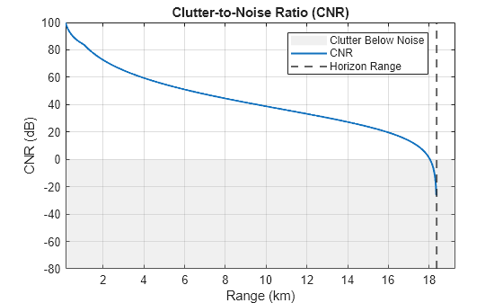
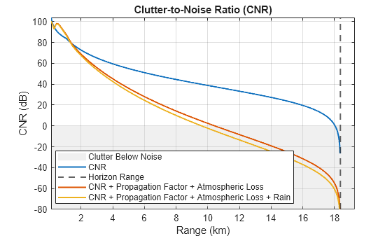
Calculate the clutter-to-noise ratio (CNR) using the radareqsnr function. Again, note the drop in CNR as the simulation range approaches the radar horizon. Calculate the range at which the clutter falls below the noise.
% Convert frequency to wavelength
lambda = freq2wavelen(freq);

% Calculate and plot the clutter-to-noise ratio
cnr = radareqsnr(lambda,Rm(:),ppow,tau,...
        'gain',[Gt Gr],'rcs',rcs,'Ts',Ts); % dB
hAxes = helperPlot(Rkm,cnr,'CNR','CNR (dB)','Clutter-to-Noise Ratio (CNR)');
ylim(hAxes,[-80 100]);
helperAddHorizLine(hAxes,Rhoriz);
helperAddBelowClutterPatch(hAxes);
% Range when clutter falls below noise
helperFindClutterBelowNoise(Rkm,cnr);
Range at which clutter falls below noise (km) = 18.04
Considering the Propagation Path
When the path between the radar and clutter deviates from free space conditions, include the clutter propagation factor and the atmospheric losses on the path. You can calculate the clutter propagation factor using the radarpropfactor function.
% Calculate radar propagation factor for clutter
Fc = radarpropfactor(Rm,freq,anht,surfht, ...
    'SurfaceHeightStandardDeviation',hgtsd,...
    'SurfaceSlope',beta0,...
    'ElevationBeamwidth',elbw);
helperPlot(Rkm,Fc,'Propagation Factor', ...
    'Propagation Factor (dB)', ...
    'One-Way Clutter Propagation Factor F_C');

Within the above plot, two propagation regions are visible:
Interference region: This is the region where reflections interfere with the direct ray. This is exhibited over the ranges where there is lobing.
Intermediate region: This is the region between the interference and diffraction region, where the diffraction region is defined as a shadow region beyond the horizon. The intermediate region, which in this example occurs at the kink in the curve at about 1.5 km, is generally estimated by an interpolation between the interference and diffraction regions.
Typically, the clutter propagation factor and the sea reflectivity are combined as the product , because measurements of surface reflectivity are generally measurements of the product rather than just the reflectivity . Calculate this product and plot the results.
% Combine clutter reflectivity and clutter propagation factor
FcLinear = db2mag(Fc); % Convert to linear units
combinedFactor = nrcs.*FcLinear.^2;
combinedFactordB = pow2db(combinedFactor);
helperPlot(Rkm,combinedFactordB,'\sigma_CF_C', ...
    '\sigma_CF_C (dB)', ...
    'One-Way Sea Clutter Propagation Factor and Reflectivity');

Next, calculate the atmospheric loss on the path using the slant-path tropopl function. Use the default standard atmospheric model for the calculation.
% Calculate one-way loss associated with atmosphere
elAng = height2el(surfht,anht,Rm); % Elevation angle (deg)
numEl = numel(elAng);
Latmos = zeros(numEl,1);
for ie = 1:numEl
    Latmos(ie,:) = tropopl(Rm(ie),freq,anht,elAng(ie));
end
helperPlot(Rkm,Latmos,'Atmospheric Loss','Loss (dB)','One-Way Atmospheric Loss');

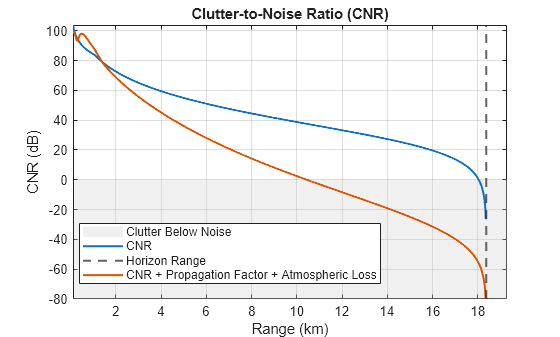
Recalculate the CNR. Include the propagation factor and atmospheric loss in the calculation. Note the change in the shape of the CNR curve. The point at which the clutter falls below the noise is much closer in range when you include these factors.
% Re-calculate CNR including radar propagation factor and atmospheric loss
cnr = radareqsnr(lambda,Rm(:),ppow,tau,...
        'gain',[Gt Gr],'rcs',rcs,'Ts',Ts, ...
        'PropagationFactor',Fc,...
        'AtmosphericLoss',Latmos); % dB
helperAddPlot(Rkm,cnr,'CNR + Propagation Factor + Atmospheric Loss',hAxes);
% Range when clutter falls below noise
helperFindClutterBelowNoise(Rkm,cnr);
Range at which clutter falls below noise (km) = 10.44
Understanding Weather Effects
Just as the atmosphere affects the detection of a target, weather also affects the detection of clutter. Consider the effect of rain over the simulated ranges. First calculate the rain attenuation.
% Calculate one-way loss associated with rain
rr = 50;                           % Rain rate (mm/h)
polAng = 0;                        % Polarization tilt angle (0 degrees for horizontal)
elAng = height2el(surfht,anht,Rm); % Elevation angle (deg)
numEl = numel(elAng);
Lrain = zeros(numEl,1);
for ie = 1:numEl
    Lrain(ie,:) = cranerainpl(Rm(ie),freq,rr,elAng(ie),polAng);
end
helperPlot(Rkm,Lrain,'Rain Loss','Loss (dB)','One-Way Rain Loss');
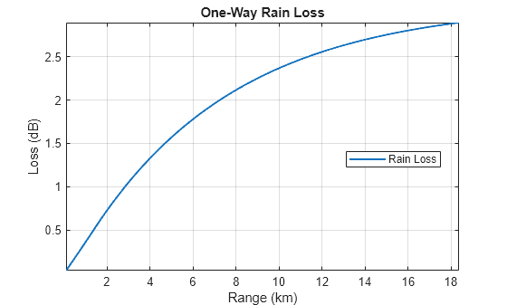
Recalculate the CNR. Include the propagation path and the rain loss. Note that there is only a slight decrease in the CNR due to the presence of the rain.
% Re-calculate CNR including radar propagation factor, atmospheric loss,
% and rain loss
cnr = radareqsnr(lambda,Rm(:),ppow,tau,...
        'gain',[Gt Gr],'rcs',rcs,'Ts',Ts, ...
        'PropagationFactor',Fc, ...
        'AtmosphericLoss',Latmos + Lrain); % dB
helperAddPlot(Rkm,cnr,'CNR + Propagation Factor + Atmospheric Loss + Rain',hAxes);
% Range when clutter falls below noise
helperFindClutterBelowNoise(Rkm,cnr);
Range at which clutter falls below noise (km) = 9.61
Summary
This example introduces concepts regarding the simulation of sea surfaces. The sea reflectivity exhibits the following properties:
A strong dependence on sea state
A proportional dependence on frequency
A dependence on polarization that decreases with increasing frequency
A strong dependence on grazing angle at low grazing angles
This example also discusses how to use the sea state physical properties and reflectivity for the calculation of the clutter-to-noise ratio for a maritime surveillance radar system. Additionally, the example explains ways to improve simulation of the propagation path.
References
Barton, David Knox. Radar Equations for Modern Radar. Artech House Radar Series. Boston, Mass: Artech House, 2013.
Blake, L. V. Machine Plotting of Radar Vertical-Plane Coverage Diagrams. NRL Report, 7098, Naval Research Laboratory, 1970.
Gregers-Hansen, V., and R. Mittal. An Improved Empirical Model for Radar Sea Clutter Reflectivity. NRL/MR, 5310-12-9346, Naval Research Laboratory, 27 Apr. 2012.
Richards, M. A., Jim Scheer, William A. Holm, and William L. Melvin, eds. Principles of Modern Radar. Raleigh, NC: SciTech Pub, 2010.
function helperPlotSeaRoughness(ss,hgtsd,beta0,vw)
% Creates 3x1 plot of sea roughness outputs

% Create figure
figure

% Plot standard deviation of sea wave height
subplot(3,1,1)
plot(ss,hgtsd,'-o','LineWidth',1.5)
ylabel([sprintf('Wave\nHeight ') '\sigma_h (m)'])
title('Sea Wave Roughness')
grid on;

% Plot sea wave slope
subplot(3,1,2)
plot(ss,beta0,'-o','LineWidth',1.5)
ylabel([sprintf('Wave\nSlope ') '\beta_0 (deg)'])
grid on;

% Plot wind velocity
subplot(3,1,3)
plot(ss,vw,'-o','LineWidth',1.5)
xlabel('Sea State')
ylabel([sprintf('Wind\nVelocity ')  'v_w (m/s)'])
grid on;
end

function hAxes = helperPlotSeaReflectivity(ss,grazAng,freq,nrcs,pol,hAxes)
% Plot sea reflectivities

% Create figure and new axes if axes are not passed in
newFigure = false;
if nargin < 6
    figure();
    hAxes = gca;
    newFigure = true;
end

% Get polarization string
switch lower(pol)
    case 'h'
        lineStyle = '-';
    otherwise
        lineStyle = '--';
end

% Plot
if numel(grazAng) == 1
    hLine = semilogx(hAxes,freq(:).*1e-9,pow2db(nrcs),lineStyle,'LineWidth',1.5);
    xlabel('Frequency (GHz)')
else
    hLine = plot(hAxes,grazAng(:),pow2db(nrcs),lineStyle,'LineWidth',1.5);
    xlabel('Grazing Angle (deg)')
end

% Set display names
numLines = size(nrcs,2);
for ii = 1:numLines
    hLine(ii).DisplayName = sprintf('SS %d, %s',ss(ii),pol);
    if newFigure
        hLine(ii).Color = brighten(hLine(ii).Color,0.5);
    end
end

% Update labels and axes
ylabel('Reflectivity \sigma_0 (dB)')
title('Sea State Reflectivity \sigma_0')
grid on
axis tight
hold on;

% Add legend
legend('Location','southoutside','NumColumns',5,'Orientation','Horizontal');
end

function varargout = helperPlot(Rkm,y,displayName,ylabelStr,titleName)
% Used in CNR analysis

% Create figure
hFig = figure;
hAxes = axes(hFig);

% Plot
plot(hAxes,Rkm,y,'LineWidth',1.5,'DisplayName',displayName);
grid(hAxes,'on');
hold(hAxes,'on');
xlabel(hAxes,'Range (km)')
ylabel(hAxes,ylabelStr);
title(hAxes,titleName);
axis(hAxes,'tight');

% Add legend
legend(hAxes,'Location','Best')

% Output axes
if nargout ~= 0
    varargout{1} = hAxes;
end
end

function helperAddPlot(Rkm,y,displayName,hAxes)
% Used in CNR analysis

% Plot
ylimsIn = get(hAxes,'Ylim');
plot(hAxes,Rkm,y,'LineWidth',1.5,'DisplayName',displayName);
axis(hAxes,'tight');
ylimsNew = get(hAxes,'Ylim');
set(hAxes,'Ylim',[ylimsIn(1) ylimsNew(2)]);
end

function helperAddHorizLine(hAxes,Rhoriz)
% Add vertical line indicating horizon range

xline(Rhoriz.*1e-3,'--','DisplayName','Horizon Range','LineWidth',1.5);
xlims = get(hAxes,'XLim');
xlim([xlims(1) Rhoriz.*1e-3*(1.05)]);
end

function helperAddBelowClutterPatch(hAxes)
% Add patch indicating when clutter falls below the noise

xlims = get(hAxes,'Xlim');
ylims = get(hAxes,'Ylim');
x = [xlims(1) xlims(1) xlims(2) xlims(2) xlims(1)];
y = [ylims(1) 0 0 ylims(1) ylims(1)];
hP = patch(hAxes,x,y,[0.8 0.8 0.8], ...
    'FaceAlpha',0.3,'EdgeColor','none','DisplayName','Clutter Below Noise');
uistack(hP,'bottom');
end

function helperFindClutterBelowNoise(Rkm,cnr)
% Find the point at which the clutter falls below the noise
idxNotNegInf = ~isinf(cnr);
Rclutterbelow = interp1(cnr(idxNotNegInf),Rkm(idxNotNegInf),0);
fprintf('Range at which clutter falls below noise (km) = %.2f\n',Rclutterbelow)
end