Train Biped Robot to Walk Using Reinforcement Learning Agents
This example shows how to train a biped robot to walk using either a deep deterministic policy gradient (DDPG) agent or a twin-delayed deep deterministic policy gradient (TD3) agent. In the example, you also compare the performance of these trained agents. The robot in this example is modeled in Simscape™ Multibody™. For more information on these agents, see Deep Deterministic Policy Gradient (DDPG) Agent and Twin-Delayed Deep Deterministic (TD3) Policy Gradient Agent.
For the purpose of comparison in this example, this example trains both agents on the biped robot environment with the same model parameters. The example also configures the agents to have the following settings in common.
Initial condition strategy of the biped robot.
Network structure of actor and critic, inspired by [1].
Options for actor and critic objects.
Training options (sample time, discount factor, mini-batch size, experience buffer length, exploration noise).
Fix Random Seed Generator to Improve Reproducibility
The example code might involve computation of random numbers at several stages. Fixing the random number stream at the beginning of some sections in the example code preserves the random number sequence in the section every time you run it, which increases the likelihood of reproducing the results. For more information, see Results Reproducibility.
Fix the random number stream with seed 0 and random number algorithm Mersenne Twister. For more information on controlling the seed used for random number generation, see rng.
previousRngState = rng(0,"twister");The output previousRngState is a structure that contains information about the previous state of the stream. You will restore the state at the end of the example.
Biped Robot Model
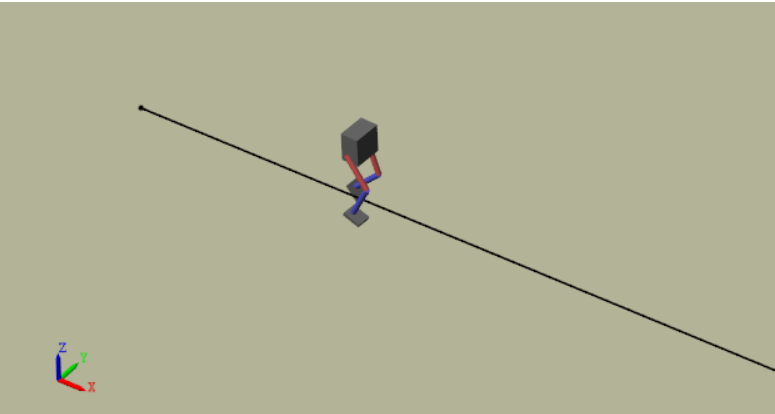
The reinforcement learning environment for this example is a biped robot. The training goal is to make the robot walk in a straight line using minimal control effort.

Load the parameters of the model into the MATLAB® workspace using the robotParametersRL Script provided in the example folder.
robotParametersRL
Open the Simulink® model.
mdl = "rlWalkingBipedRobot";
open_system(mdl)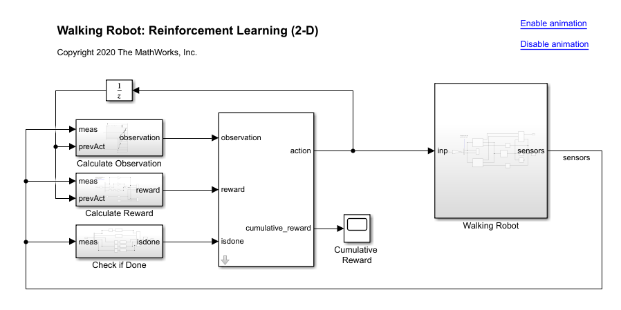
The robot is modeled using Simscape™ Multibody™.
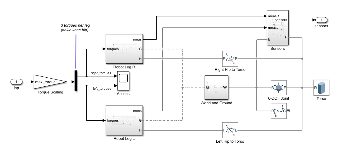
In this model:
In the neutral 0 rad position, both of the legs are straight and the ankles are flat.
The foot contact is modeled using the Spatial Contact Force (Simscape Multibody) block.
The agent can control 3 individual joints (ankle, knee, and hip) on both legs of the robot by applying torque signals from -3 to 3 N·m. The actual computed action signals are normalized between -1 and 1.
The environment provides the following 29 observations to the agent.
Y (lateral) and Z (vertical) translations of the torso center of mass. The translation in the Z direction is normalized to a similar range as the other observations.
X (forward), Y (lateral), and Z (vertical) translation velocities.
Yaw, pitch, and roll angles of the torso.
Yaw, pitch, and roll angular velocities of the torso.
Angular positions and velocities of the three joints (ankle, knee, hip) on both legs.
Action values from the previous time step.
The episode terminates if either of the following conditions occur.
The robot torso center of mass is less than 0.1 m in the Z direction (the robot falls) or more than 1 m in the either Y direction (the robot moves too far to the side).
The absolute value of either the roll, pitch, or yaw is greater than 0.7854 rad.
The following reward function , which is provided at every time step is inspired by [2].
Here:
is the translation velocity in the X direction (forward toward goal) of the robot.
is the lateral translation displacement of the robot from the target straight line trajectory.
is the normalized vertical translation displacement of the robot center of mass.
is the torque from joint i from the previous time step.
is the sample time of the environment.
is the final simulation time of the environment.
This reward function encourages the agent to move forward by providing a positive reward for positive forward velocity. It also encourages the agent to avoid episode termination by providing a constant reward () at every time step. The other terms in the reward function are penalties for substantial changes in lateral and vertical translations, and for the use of excess control effort.
Create Environment Object
Create the observation specification.
numObs = 29;
obsInfo = rlNumericSpec([numObs 1]);
obsInfo.Name = "observations";
Create the action specification.
numAct = 6;
actInfo = rlNumericSpec([numAct 1],LowerLimit=-1,UpperLimit=1);
actInfo.Name = "foot_torque";
Create the environment object for the walking robot model.
blk = mdl + "/RL Agent";Specify the helper function walkerResetFcn as the reset function for the environment. For more information, see Reset Function for Simulink Environments.
env = rlSimulinkEnv(mdl,blk,obsInfo,actInfo);
env.ResetFcn = @(in) walkerResetFcn(in, ...
    upper_leg_length/100, ...
    lower_leg_length/100, ...
    h/100);
Select and Create Agent for Training
When you create the agent, the initial parameters of the actor and critic networks are initialized with random values. Fix the random number stream so that the agent is always initialized with the same parameter values.
rng(0,"twister");This example provides the option to train the robot using either a DDPG or TD3 agent. To simulate the robot with the agent of your choice, set the AgentSelection flag accordingly.
AgentSelection ="DDPG"; switch AgentSelection case "DDPG" agent = createDDPGAgent(numObs,obsInfo,numAct,actInfo,Ts); case "TD3" agent = createTD3Agent(numObs,obsInfo,numAct,actInfo,Ts); otherwise disp("Assign AgentSelection to DDPG or TD3") end
The createDDPGAgent and createTD3Agent helper functions (provided in the example folder) perform the following actions.
Create actor and critic networks.
Specify options for actors and critics.
Create actors and critics using the networks and options previously created.
Configure agent specific options.
Create the agent.
DDPG Agent
DDPG agents use a parameterized deterministic policy over continuous action spaces, which is learned by a continuous deterministic actor, and a parameterized Q-value function approximator to estimate the value of the policy. Use neural networks to model both the policy and the Q-value function. The actor and critic networks for this example are inspired by [1].
For details on how the DDPG agent is created, see the createDDPGAgent helper function. For information on configuring DDPG agent options, see rlDDPGAgentOptions.
For more information on creating a deep neural network value function representation, see Create Actors, Critics, and Policy Objects. For an example that creates neural networks for DDPG agents, see Compare DDPG Agent to LQR Controller.
TD3 Agent
The critic of a DDPG agent can overestimate the Q value. Because the agent uses the Q value to update its policy (actor), the resultant policy can be suboptimal and can accumulate training errors that can lead to divergent behavior. The TD3 algorithm is an extension of DDPG with improvements that make it more robust by preventing overestimation of Q values [3].
Two critic networks — TD3 agents learn two critic networks independently and use the minimum value function estimate to update the actor (policy). Doing so prevents accumulation of error in subsequent steps and overestimation of Q values.
Addition of target policy noise — Adding clipped noise to value functions smooths out Q function values over similar actions. Doing so prevents learning an incorrect sharp peak of noisy value estimate.
Delayed policy and target updates — For a TD3 agent, delaying the actor network update allows more time for the Q function to reduce error (get closer to the required target) before updating the policy. Doing so prevents variance in value estimates and results in a higher quality policy update. This example sets the policy and target frequency options to
1as to better compare the impact of two critic networks and target policy noise between the DDPG and TD3 agents.
The structure of the actor and critic networks used for this agent are the same as the ones used for DDPG agent. For details on the creation of the TD3 agent, see the createTD3Agent helper function. For information on configuring TD3 agent options, see rlTD3AgentOptions.
Get the actor and critic neural networks from the agent.
actor = getActor(agent);
critic = getCritic(agent);
actorNet = getModel(actor);
criticNet = getModel(critic(1));
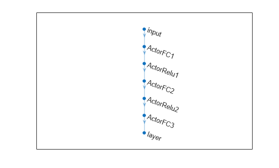
View a summary and plot of the actor neural network.
summary(actorNet);
   Initialized: true

   Number of learnables: 134.1k

   Inputs:
      1   'input'   29 features
plot(actorNet);
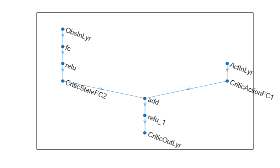
View a summary and plot of the critic neural network.
summary(criticNet);
   Initialized: true

   Number of learnables: 134.7k

   Inputs:
      1   'ObsInLyr'   29 features
      2   'ActInLyr'   6 features
plot(criticNet);
Specify Training Options and Train Agent
For this example, the training options for the DDPG and TD3 agents are the same.
Run each training session for 3000 episodes with each episode lasting at most
maxStepstime steps.Terminate the training only when it reaches the maximum number of episodes (
maxEpisodes) by settingStopTrainingCriteriato"none". Doing so allows the comparison of the learning curves for multiple agents over the entire training session.
For more information and additional options, see rlTrainingOptions.
maxEpisodes = 3000;
maxSteps = floor(Tf/Ts);
trainOpts = rlTrainingOptions( ...
    MaxEpisodes=maxEpisodes, ...
    MaxStepsPerEpisode=maxSteps, ...
    ScoreAveragingWindowLength=250, ...
    StopTrainingCriteria="none", ...
    SimulationStorageType="file", ...
    SaveSimulationDirectory=AgentSelection+"Sims");
To train the agent in parallel, specify the following training options. Training in parallel requires Parallel Computing Toolbox™. If you do not have Parallel Computing Toolbox software installed, set UseParallel to false.
Set the
UseParalleloption to true.Train the agent in parallel asynchronously.
trainOpts.UseParallel =true; trainOpts.ParallelizationOptions.Mode =
"async";
In parallel training, workers simulate the agent's policy with the environment and store experiences in the replay memory. When workers operate asynchronously the order of stored experiences might not be deterministic and can ultimately make the training results different. To maximize the reproducibility likelihood:
Initialize the parallel pool with the same number of parallel workers every time you run the code. For information on specifying the pool size see Discover Clusters and Use Cluster Profiles (Parallel Computing Toolbox).
Use synchronous parallel training by setting
trainOpts.ParallelizationOptions.Modeto"sync".Assign a random seed to each parallel worker using
trainOpts.ParallelizationOptions.WorkerRandomSeeds. The default value of -1 assigns a unique random seed to each parallel worker.
Fix the random stream for reproducibility.
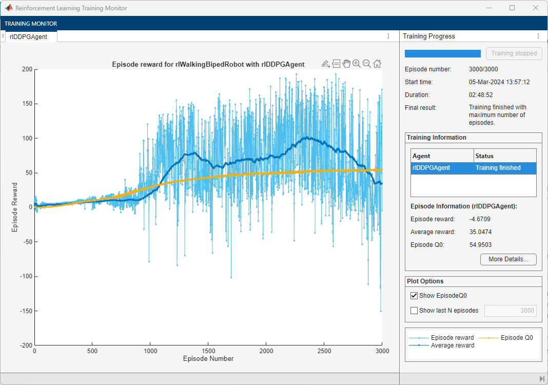
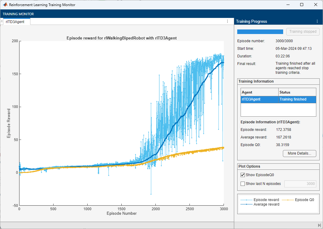
rng(0,"twister");Train the agent using the train function. This process is computationally intensive and takes several hours to complete for each agent. To save time while running this example, load a pretrained agent by setting doTraining to false. To train the agent yourself, set doTraining to true. Due to randomness in the parallel training, you can expect different training results from the plots that follow. The pretrained agents were trained in parallel using four workers.
doTraining =false; if doTraining % Train the agent. trainingStats = train(agent,env,trainOpts); else % Load a pretrained agent for the selected agent type. if strcmp(AgentSelection,"DDPG") load(fullfile("DDPGAgent","run1.mat"),"agent") else load(fullfile("TD3Agent","run1.mat"),"agent") end end
Simulate Trained Agents
Fix the random stream for reproducibility.
rng(0,"twister");To validate the performance of the trained agent, simulate it within the biped robot environment. For more information on agent simulation, see rlSimulationOptions and sim.
simOptions = rlSimulationOptions(MaxSteps=maxSteps);
experience = sim(env,agent,simOptions);
Compare Agent Performance
For the following agent comparison, each agent was trained five times using a different random seed each time. Due to the random exploration noise and the randomness in the parallel training, the learning curve for each run is different. Because the training of agents for multiple runs can take several days to complete, this comparison uses pretrained agents.
For the DDPG and TD3 agents, plot the average and standard deviation of the episode reward (top plot) and the episode Q0 value (bottom plot). The episode Q0 value is the critic estimate of the discounted long-term reward at the start of each episode given the initial observation of the environment. For a well-designed critic, the episode Q0 value approaches the true discounted long-term reward.
Fix the random stream for reproducibility.
rng(0,"twister");Compare the performance of the pretrained agents using data stored in the DDPGAgent and TD3Agent folders. To plot the performance metrics, specify the folder names as input arguments to the comparePerformance function. The comparison data and the function are found in the example directory.
comparePerformance("DDPGAgent","TD3Agent")
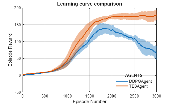

Based on the Learning curve comparison plot:
The DDPG agent can pick up learning faster than the TD3 agent in some cases, however the DDPG agent tends to have inconsistent long-term training performance.
The TD3 agent consistently learns satisfactory walking policies for the environment and tends to show better convergence properties compared to DDPG.
Based on the Episode Q0 comparison plot:
The TD3 agent more conservatively estimates the discounted long-term reward compared to DDPG. This is because TD3 estimates the discounted long-term reward as the minimum of the values approximated from the two critics.
For another example on how to train a humanoid robot to walk using a DDPG agent, see Train Humanoid Walker (Simscape Multibody). For an example on how to train a quadruped robot to walk using a DDPG agent, see Quadruped Robot Locomotion Using DDPG Agent.
Restore the random number stream using the information stored in previousRngState.
rng(previousRngState);
References
[1] Lillicrap, Timothy P., Jonathan J. Hunt, Alexander Pritzel, Nicolas Heess, Tom Erez, Yuval Tassa, David Silver, and Daan Wierstra. "Continuous Control with Deep Reinforcement Learning." Preprint, submitted July 5, 2019. https://arxiv.org/abs/1509.02971.
[2] Heess, Nicolas, Dhruva TB, Srinivasan Sriram, Jay Lemmon, Josh Merel, Greg Wayne, Yuval Tassa, et al. "Emergence of Locomotion Behaviours in Rich Environments." Preprint, submitted July 10, 2017. https://arxiv.org/abs/1707.02286.
[3] Fujimoto, Scott, Herke van Hoof, and David Meger. "Addressing Function Approximation Error in Actor-Critic Methods." Preprint, submitted October 22, 2018. https://arxiv.org/abs/1802.09477.
See Also
Functions
train|sim|rlSimulinkEnv
Objects
rlDDPGAgent|rlDDPGAgentOptions|rlTD3Agent|rlTD3AgentOptions|rlQValueFunction|rlContinuousDeterministicActor|rlOptimizerOptions|rlTrainingOptions|rlSimulationOptions
Blocks
Topics
- Train AC Agent to Balance Discrete Cart-Pole Using Parallel Computing
- Train DQN Agent for Lane Keeping Assist Using Parallel Computing
- Quadruped Robot Locomotion Using DDPG Agent
- Add Safety Constraint to Simulate Two-Link Robot with SAC Agent
- Define Observation and Reward Signals in Custom Environments
- Deep Deterministic Policy Gradient (DDPG) Agent
- Twin-Delayed Deep Deterministic (TD3) Policy Gradient Agent
- Train Agents Using Parallel Computing and GPUs