Test, Visualize, and Enforce Passivity of Rational Output

This example shows how to test, visualize, and enforce the passivity of output from the rational function.

S-Parameter Data Passivity

Time-domain analysis and simulation depend critically on the ability to convert frequency-domain S-parameter data into causal, stable, and passive time-domain representations. Because the rational function guarantees that all poles are in the left half plane, rational output is both stable and causal by construction. The problem is passivity.

N-port S-parameter data represents a frequency-dependent transfer function H(f). You can create an S-parameters object in RF Toolbox™ by reading a Touchstone file, such as passive.s2p, into the sparameters function.

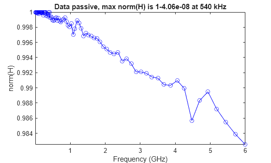
You can use the ispassive function to check the passivity of the S-parameter data, and the passivity function to plot the 2-norm of the N-by-N matrices H(f) at each data frequency.

S = sparameters("passive.s2p");
ispassive(S)

ans = logical
   1

passivity(S)

Testing and Visualizing rational Output Passivity

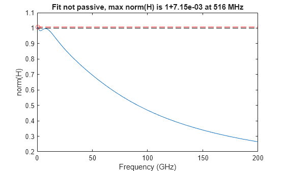
The rational function converts N-port S-parameter data, S, into an object that represents a rational fit to the data. Using the ispassive function on the output reports that even if input data S is passive, the output fit is not passive. In other words, the norm H(f) is greater than 1 at some frequency in the range [0,Inf].

The passivity function takes the output of the rational function as input and plots its passivity. This is a plot of the upper bound of the norm(H(f)) on [0,Inf], also known as the H-infinity norm.

fit = rational(S);
ispassive(fit)

ans = logical
   0

passivity(fit)

The makepassive function takes as input a rational object, and produces a passive fit by using convex optimization techniques to optimally match the data of the S-parameter input S while satisfying passivity constraints. The residues and direct term of the output pfit are modified, but the poles of the output pfit are identical to the poles of the input fit.

pfit = makepassive(fit,'Display','on');

Iter	H-infinity norm	Frequency	Error (dB)	Constraints
0		1+7.15e-03		516 MHz		-40.4597
1		1+5.44e-04		319 MHz		-41.7549	5
2		1+7.78e-05		383 MHz		-41.7318	7
3		1+8.20e-06		360 MHz		-41.7275	9
4		1-8.74e-07		359 MHz		-41.7272	10

ispassive(pfit)

ans = logical
   1

passivity(pfit)

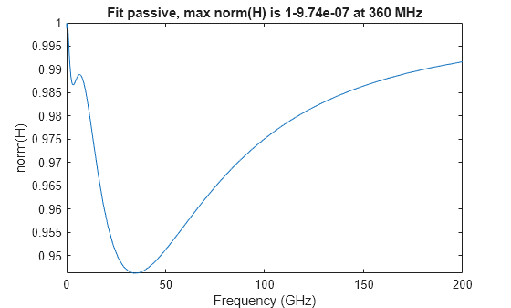
all(pfit.Poles == fit.Poles)

ans = logical
   1

Generate Equivalent SPICE Circuit from Passive Fit

The generateSPICE function takes a passive fit and generates an equivalent circuit as a SPICE subcircuit file. The input fit is an object as returned by rational with an S-parameters object as input. The generated file is a SPICE model constructed solely of passive R, L, C elements and controlled source elements E, F, G, and H.

generateSPICE(pfit,'mypassive.ckt')
type mypassive.ckt

* Equivalent circuit model for mypassive.ckt
.SUBCKT mypassive po1 po2
Vsp1 po1 p1 0
Vsr1 p1 pr1 0
Rp1 pr1 0 50
Ru1 u1 0 50
Fr1 u1 0 Vsr1 -1
Fu1 u1 0 Vsp1 -1
Ry1 y1 0 1
Gy1 p1 0 y1 0 -0.02
Vsp2 po2 p2 0
Vsr2 p2 pr2 0
Rp2 pr2 0 50
Ru2 u2 0 50
Fr2 u2 0 Vsr2 -1
Fu2 u2 0 Vsp2 -1
Ry2 y2 0 1
Gy2 p2 0 y2 0 -0.02
Rx1 x1 0 1
Fxc1_2 x1 0 Vx2 1.73989373346879
Cx1 x1 xm1 4.40797252207916e-09
Vx1 xm1 0 0
Gx1_1 x1 0 u1 0 -0.0637715388486617
Rx2 x2 0 1
Fxc2_1 x2 0 Vx1 -1.10431281974679
Cx2 x2 xm2 4.40797252207916e-09
Vx2 xm2 0 0
Gx2_1 x2 0 u1 0 0.0704237278855573
Rx3 x3 0 1
Cx3 x3 0 2.46549216562577e-12
Gx3_1 x3 0 u1 0 -0.857318903882464
Rx4 x4 0 1
Cx4 x4 0 1.19630315229193e-11
Gx4_1 x4 0 u1 0 -2.76951576517327
Rx5 x5 0 1
Cx5 x5 0 1.85575922991507e-11
Gx5_1 x5 0 u1 0 -1.31129739149988
Rx6 x6 0 1
Cx6 x6 0 8.71015575460466e-11
Gx6_1 x6 0 u1 0 -0.691516260248889
Rx7 x7 0 1
Cx7 x7 0 5.76402180365138e-10
Gx7_1 x7 0 u1 0 -0.0721111836946592
Rx8 x8 0 1
Cx8 x8 0 1.3287059941001e-08
Gx8_1 x8 0 u1 0 -0.853435063811975
Rx9 x9 0 1
Fxc9_10 x9 0 Vx10 1.74905636890478
Cx9 x9 xm9 4.40797252207916e-09
Vx9 xm9 0 0
Gx9_2 x9 0 u2 0 -0.0646370023478586
Rx10 x10 0 1
Fxc10_9 x10 0 Vx9 -1.09852774846234
Cx10 x10 xm10 4.40797252207916e-09
Vx10 xm10 0 0
Gx10_2 x10 0 u2 0 0.0710055406565479
Rx11 x11 0 1
Cx11 x11 0 2.46549216562577e-12
Gx11_2 x11 0 u2 0 -0.903135528297918
Rx12 x12 0 1
Cx12 x12 0 1.19630315229193e-11
Gx12_2 x12 0 u2 0 -2.78929031830451
Rx13 x13 0 1
Cx13 x13 0 1.85575922991507e-11
Gx13_2 x13 0 u2 0 -1.32148208547721
Rx14 x14 0 1
Cx14 x14 0 8.71015575460466e-11
Gx14_2 x14 0 u2 0 -0.731803256468193
Rx15 x15 0 1
Cx15 x15 0 5.76402180365138e-10
Gx15_2 x15 0 u2 0 -0.0762131540132594
Rx16 x16 0 1
Cx16 x16 0 1.3287059941001e-08
Gx16_2 x16 0 u2 0 -0.853729456884103
Gyc1_1 y1 0 x1 0 -1
Gyc1_2 y1 0 x2 0 -1
Gyc1_3 y1 0 x3 0 -1
Gyc1_4 y1 0 x4 0 0.133850507926629
Gyc1_5 y1 0 x5 0 -0.577037380579007
Gyc1_6 y1 0 x6 0 -1
Gyc1_7 y1 0 x7 0 1
Gyc1_8 y1 0 x8 0 0.998948943573286
Gyc1_9 y1 0 x9 0 0.981453226199042
Gyc1_10 y1 0 x10 0 0.985620343832744
Gyc1_11 y1 0 x11 0 0.820911611991671
Gyc1_12 y1 0 x12 0 -1
Gyc1_13 y1 0 x13 0 1
Gyc1_14 y1 0 x14 0 0.920286989392691
Gyc1_15 y1 0 x15 0 -0.916745641088617
Gyc1_16 y1 0 x16 0 -1
Gyd1_1 y1 0 u1 0 0.999439185502022
Gyd1_2 y1 0 u2 0 -0.0124599724327471
Gyc2_1 y2 0 x1 0 0.992914839827891
Gyc2_2 y2 0 x2 0 0.990615905520051
Gyc2_3 y2 0 x3 0 0.82366068414698
Gyc2_4 y2 0 x4 0 -1
Gyc2_5 y2 0 x5 0 1
Gyc2_6 y2 0 x6 0 0.974340220890268
Gyc2_7 y2 0 x7 0 -0.968867916185466
Gyc2_8 y2 0 x8 0 -1
Gyc2_9 y2 0 x9 0 -1
Gyc2_10 y2 0 x10 0 -1
Gyc2_11 y2 0 x11 0 -1
Gyc2_12 y2 0 x12 0 0.207642941515442
Gyc2_13 y2 0 x13 0 -0.66809244556828
Gyc2_14 y2 0 x14 0 -1
Gyc2_15 y2 0 x15 0 1
Gyc2_16 y2 0 x16 0 0.998712525623536
Gyd2_1 y2 0 u1 0 0.012810453976459
Gyd2_2 y2 0 u2 0 0.999536586117702
.ENDS