Measure Transition Risk for Loan Portfolios Based on Climate Scenarios with Paths

Open Live Script

This example shows the effect of transition risk on portfolios of loans from two banks under two different climate scenarios. In this example, each climate scenario uses 400 simulations and the visualizations reflect a distribution of portfolio outcomes.

Download and Import Climate Data

This example uses climate scenario data from the MIT Joint Program on the Science and Policy of Global Change. For details about this freely available data, see the MIT data repository.

Download the raw data from the MathWorks® support files area.

filename = matlab.internal.examples.downloadSupportFile("risk","MITUncertaintyData.zip");

Make a folder in your current directory for the climate data.

if not(isfolder("MITUncertaintyData"))
    mkdir("MITUncertaintyData")
end

Unzip the downloaded files into the created folder.

MITDataFolder = fullfile(pwd,"MITUncertaintyData");
unzip(filename,MITDataFolder)

The data set has three climate scenarios. The Scenario_Descriptions.docx file provides a description of the scenarios.

scenarios = ["1.5C","2C","Ref"];

Read the climate data into MATLAB® by using the helper function importClimateData in a for–loop.

energies = ["Coal" "Gas" "Oil" "Nuclear" "Hydro" "Biomass" "Renewables"];
regions = ["GLB" "USA" "CAN" "MEX" "JPN" "ANZ" "EUR" "ROE" "RUS" "ASI" "CHN" "IND" "BRA" "AFR" "MES" "LAM" "REA" "KOR" "IDZ"];

climateDataDictionary = dictionary;

for scenario = scenarios
    for energy = energies
        for region = regions
            key = strcat(scenario, energy, region);
            climateDataDictionary{key} = importClimateData(scenario, energy, region);
        end
    end
end

Stack the scenarios into a tall data set.

vals = values(climateDataDictionary);
allClimateData = vertcat(vals{:});
allClimateData.Year = str2double(cellstr(allClimateData.Year));
head(allClimateData)

    Simulation    Year    Energy Use    Scenario    Region    Energy
    __________    ____    __________    ________    ______    ______

        1         2020      151.31        1.5C       GLB       Coal 
        1         2025      137.82        1.5C       GLB       Coal 
        1         2030      135.75        1.5C       GLB       Coal 
        1         2035      14.962        1.5C       GLB       Coal 
        1         2040      18.553        1.5C       GLB       Coal 
        1         2045      33.185        1.5C       GLB       Coal 
        1         2050      42.375        1.5C       GLB       Coal 
        1         2055      40.205        1.5C       GLB       Coal

Process Climate Data

Use the climateScenario function to create a climateScenario object from the climate data.

cs = climateScenario(allClimateData, "VariableVar", "Energy", "ValueVar", "Energy Use", "CustomIdentifierVars", "Simulation")

cs = 
  climateScenario with properties:

          Identifiers: ["Region"    "Variable"    "Scenario"    "Year"    "Simulation"]
    CustomIdentifiers: "Simulation"
     IdentifierValues: [1×1 struct]

Create a new variable, Total, to represent the total primary energy use. Use the sumVariables function to compute the total energy.

energyVars = ["Coal", "Gas", "Oil", "Nuclear", "Hydro", "Biomass", "Renewables"];
cs = sumVariables(cs, energyVars, "NewVariable", "Total");

Next, use the divideVariables function to compute the market share for each energy type by using Total as the denominator.

marketShareVars = energyVars + "MarketShare";
cs = divideVariables(cs, energyVars, "Total", "NewVariables", marketShareVars);

Define the market share shock. For more details on this definition, see Profitability and Shocks on Market Share.

Let $m_{S, R} (P, t^{*})$ denote the market share at time $t^{*}$ of sector $S$ in the region $R$ in scenario $P$ . Define $m_{S, R} (B, t^{*})$ similarly. Then, the market share shock $u_{S, R} (P, B, t^{*})$ is defined as

$u_{S, R} (P, B, t^{*}) = \frac{m_{S, R} (P, t^{*}) - m_{S, R} (B, t^{*})}{m_{S, R} (B, t^{*})} .$

Compute the shocks by using the shockVariables function.

cs = shockVariables(cs, "Ref", "Variable", marketShareVars, "Scenario", ["1.5C", "2C"]);

Use the query function to extract the shocked market share variables. Then, use these variables to shock the credit risk of a portfolio of loans.

shockedVars = marketShareVars + " Shocked Against Ref";
climateData = query(cs, "Variable", shockedVars, "UnstackIdentifier", "Scenario");
head(climateData)

    Simulation    Year    Region                  Energy                     x1_5C          x2C    
    __________    ____    ______    ___________________________________    __________    __________

        1         2020     GLB      CoalMarketShare Shocked Against Ref    -0.0071761    -0.0071761
        1         2025     GLB      CoalMarketShare Shocked Against Ref     -0.063951     -0.063951
        1         2030     GLB      CoalMarketShare Shocked Against Ref     -0.074431     -0.074431
        1         2035     GLB      CoalMarketShare Shocked Against Ref      -0.78883       -0.2633
        1         2040     GLB      CoalMarketShare Shocked Against Ref      -0.70596      -0.38786
        1         2045     GLB      CoalMarketShare Shocked Against Ref      -0.45511      -0.56811
        1         2050     GLB      CoalMarketShare Shocked Against Ref      -0.30711      -0.40091
        1         2055     GLB      CoalMarketShare Shocked Against Ref      -0.32543      -0.17114

Relabel the data for convenience.

climateData.Energy = categorical(replace(cellstr(climateData.Energy), "MarketShare Shocked Against Ref", ""));
climateData = renamevars(climateData, ["x1_5C", "x2C"], ["Shock1_5C", "Shock2C"]);

The maximum negative shock is –1. Note that the maximum positive shock is Inf. Cap the positive shock so that the maximum positive shock has magnitude 1.

climateData.Shock1_5CCap = min(climateData.Shock1_5C, 1);
climateData.Shock2CCap = min(climateData.Shock2C, 1);
head(climateData)

    Simulation    Year    Region    Energy    Shock1_5C      Shock2C      Shock1_5CCap    Shock2CCap
    __________    ____    ______    ______    __________    __________    ____________    __________

        1         2020     GLB       Coal     -0.0071761    -0.0071761     -0.0071761     -0.0071761
        1         2025     GLB       Coal      -0.063951     -0.063951      -0.063951      -0.063951
        1         2030     GLB       Coal      -0.074431     -0.074431      -0.074431      -0.074431
        1         2035     GLB       Coal       -0.78883       -0.2633       -0.78883        -0.2633
        1         2040     GLB       Coal       -0.70596      -0.38786       -0.70596       -0.38786
        1         2045     GLB       Coal       -0.45511      -0.56811       -0.45511       -0.56811
        1         2050     GLB       Coal       -0.30711      -0.40091       -0.30711       -0.40091
        1         2055     GLB       Coal       -0.32543      -0.17114       -0.32543       -0.17114

Process Portfolio Data

To process the portfolio data, you use a simulation that is similar to the one in Measure Transition Risk for Loan Portfolios with Respect to Climate Scenarios, but this simulation has more granular regions and additional simulated loan-level data.

First, load the data.

load("ClimateLoanPortfolioDataGranular.mat")
ClimateLoanPortfolioDataGranular.BorrowerSector = renamecats(ClimateLoanPortfolioDataGranular.BorrowerSector,["Bioenergy", "Renewables (wind&solar)"],["Biomass","Renewables"]);

Generate histograms to show the distribution of loans by region and sector for the two simulated banks.

LoanPortfolioDataBank1 = ClimateLoanPortfolioDataGranular(ClimateLoanPortfolioDataGranular.Bank=="Bank1",:);
LoanPortfolioDataBank2 = ClimateLoanPortfolioDataGranular(ClimateLoanPortfolioDataGranular.Bank=="Bank2",:);

[CountsRegion1, BinsRegion1] = histcounts(LoanPortfolioDataBank1.GranularBorrowerRegion);
[CountsSector1, BinsSector1] = histcounts(LoanPortfolioDataBank1.BorrowerSector);
[CountsRegion2, BinsRegion2] = histcounts(LoanPortfolioDataBank2.GranularBorrowerRegion);
[CountsSector2, BinsSector2] = histcounts(LoanPortfolioDataBank2.BorrowerSector);

figure
tiledlayout(2,1)
nexttile
b1 = barh(categorical(BinsRegion1), [CountsRegion1; CountsRegion2], "FaceColor", "flat");
xlabel("Loans")
ylabel("Regions")
title("Distribution of Regions")
legend(["Bank 1", "Bank 2"],"Location","best")
b1(1).CData = [0.633, 0.078, 0.243];
b1(2).CData = [0.467, 0.675, 0.188];
fig = gcf;
currentPosition = get(fig, 'Position');
newHeight = currentPosition(4) * 2;
set(fig, 'Position', [currentPosition(1), currentPosition(2), currentPosition(3), newHeight]);

nexttile
b2 = barh(categorical(BinsSector1), [CountsSector1; CountsSector2], "FaceColor", "flat");
xlabel("Loans")
ylabel("Sectors")
title("Distribution of Sectors")
legend(["Bank 1", "Bank 2"],"Location","best")
b2(1).CData = [0.633, 0.078, 0.243];
b2(2).CData = [0.467, 0.675, 0.188];

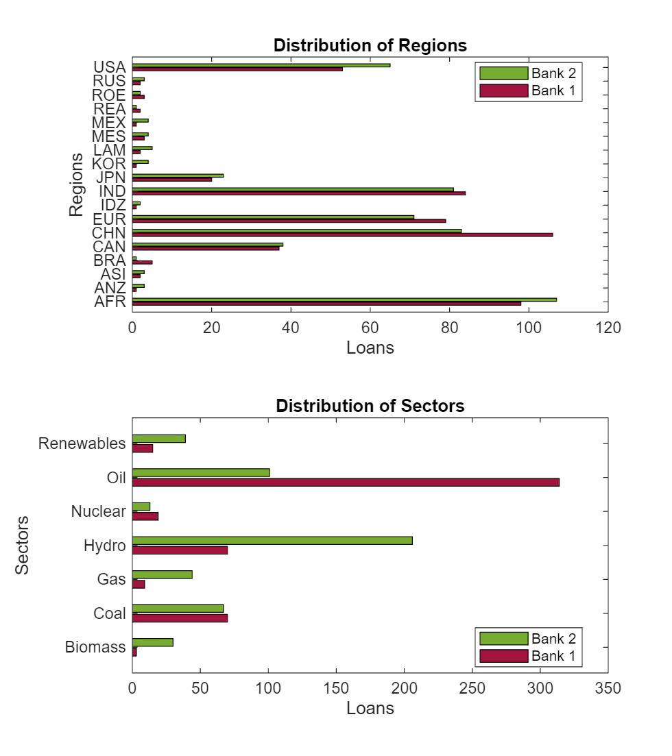
Figure contains 2 axes objects. Axes object 1 with title Distribution of Regions, xlabel Loans, ylabel Regions contains 2 objects of type bar. These objects represent Bank 1, Bank 2. Axes object 2 with title Distribution of Sectors, xlabel Loans, ylabel Sectors contains 2 objects of type bar. These objects represent Bank 1, Bank 2.

Bank 1 is heavily invested in oil fossil fuel projects, whereas Bank 2 is heavily invested in hydro green energy products. Regarding the geographical distribution of projects, both banks are similar, with a larger number of projects in developing regions like China, India, and Africa. Because Bank 2 requires a faster transition away from fossil fuels, it is likely to outperform Bank 1 more quickly in the 1.5C scenario than in the 2C scenario.

The portfolio represents a snapshot taken on December 31, 2020. This implies a static balance sheet during the time horizon, which might not be realistic. You can use a dynamic balance sheet in this step to analyze different portfolio evolution scenarios. Create a data set that represents the same portfolio with snapshots at five-year intervals from 2020 to 2095.

portfolioSnapshots = dictionary;
for year = 2020:5:2095
    value = ClimateLoanPortfolioDataGranular;
    value.Snapshot = repmat(year,height(ClimateLoanPortfolioDataGranular),1);
    portfolioSnapshots{year} = value;
end

portfolioSnapshots = vertcat(portfolioSnapshots.values{:});

Compute Change in Valuation

Create a large data set that contains each loan and snapshot with the 400 shocks by performing an outer join between the portfolio snapshots and climate data.

portfolioSnapshotsClimateData = outerjoin(portfolioSnapshots,climateData,"Type","left",...
    "LeftKeys",["BorrowerSector", "GranularBorrowerRegion", "Snapshot"],...
    "RightKeys",["Energy", "Region", "Year"]);

Calculate the loan level changes in the probability of default (PD) and valuation by using the following equations derived in Borrower's Default Conditions and Climate Policy Shocks.

$Δ p_{j} (P, B) = - χ u_{S, R} (P, B, t *) \frac{E_{j} (t_{0})}{δ_{j}}$

$Δ V_{j} (t_{0}, P, B) = - F_{j} (1 - r_{j}) Δ p_{j} (P, B)$ .

Assume that $χ = 1$ , $r_{j} = 0$ , and that $δ_{j}$ controls the size of the exogenous shock $η_{j}$ . Because the exogenous shock is independent of climate shock, you can choose it independently of the simulation. It suffices to let $δ_{j}$ be the maximum over each loan ID and snapshot pair of the quantity $2 E_{j} (t_{0}) (1 + a b s (u_{S, R} (P, B, t^{*})))$ derived in Profitability and Shocks on Market Share.

Next, compute the observation level $δ_{j}$ .

portfolioSnapshotsClimateData.deltajTemp1_5C = 2 .* portfolioSnapshotsClimateData.BookValue .* (1 + abs(portfolioSnapshotsClimateData.Shock1_5CCap));
portfolioSnapshotsClimateData.deltajTemp2C = 2 .* portfolioSnapshotsClimateData.BookValue .* (1 + abs(portfolioSnapshotsClimateData.Shock2CCap));

Find the maximum over each loan ID and snapshot pair, which is independent of the scenario and simulation.

deltaTableTemp = grpstats(portfolioSnapshotsClimateData, ...
    ["LoanID", "Snapshot"], "max", ...
    "DataVars", ["deltajTemp1_5C", "deltajTemp2C"]);
deltaTableJoin = table;
deltaTableJoin.LoanID = deltaTableTemp.LoanID;
deltaTableJoin.Snapshot = deltaTableTemp.Snapshot;
deltaTableJoin.deltaj1_5C = deltaTableTemp.max_deltajTemp1_5C;
deltaTableJoin.deltaj2C = deltaTableTemp.max_deltajTemp2C;

Join the $δ_{j}$ values back to the main data set.

portfolioSnapshotsClimateData = outerjoin(portfolioSnapshotsClimateData, ...
    deltaTableJoin, "MergeKeys", true, "Type", "left");
portfolioSnapshotsClimateData.pdChange1_5C = -portfolioSnapshotsClimateData.Shock1_5CCap .* portfolioSnapshotsClimateData.BookValue ./ portfolioSnapshotsClimateData.deltajTemp1_5C;
portfolioSnapshotsClimateData.pdChange2C = -portfolioSnapshotsClimateData.Shock2CCap .* portfolioSnapshotsClimateData.BookValue ./ portfolioSnapshotsClimateData.deltajTemp2C;
portfolioSnapshotsClimateData.valChange1_5C = -portfolioSnapshotsClimateData.FaceValue .* portfolioSnapshotsClimateData.pdChange1_5C;
portfolioSnapshotsClimateData.valChange2C = -portfolioSnapshotsClimateData.FaceValue .* portfolioSnapshotsClimateData.pdChange2C;

Aggregate the valuation changes by bank, snapshot, and simulation.

valChangeSummary = groupsummary(portfolioSnapshotsClimateData, ...
    ["Bank","Snapshot","Simulation"], "sum", ...
    ["FaceValue","valChange1_5C","valChange2C"]);
valChangeSummary.percentChangeVal1_5C = 100 * valChangeSummary.sum_valChange1_5C ./ valChangeSummary.sum_FaceValue;
valChangeSummary.percentChangeVal2C = 100 * valChangeSummary.sum_valChange2C ./ valChangeSummary.sum_FaceValue;

valChangeSummary = removevars(valChangeSummary, ...
    ["GroupCount","sum_FaceValue","sum_valChange1_5C","sum_valChange2C"]);

Calculate percentiles for the valuation changes.

valChangePrctiles = groupsummary(valChangeSummary, ...
    ["Bank","Snapshot"], ...
    {@(y) prctile(y,5), @(y) prctile(y,50), @(y) prctile(y,95)});

% Rename the percentile variables
valChangePrctiles = renamevars(valChangePrctiles, ...
    ["fun1_percentChangeVal1_5C", ...
    "fun2_percentChangeVal1_5C", ...
    "fun3_percentChangeVal1_5C", ...
    "fun1_percentChangeVal2C", ...
    "fun2_percentChangeVal2C", ...
    "fun3_percentChangeVal2C"], ...
    ["percentChangeVal1_5C_5", ...
    "percentChangeVal1_5C_50", ...
    "percentChangeVal1_5C_95", ...
    "percentChangeVal2C_5", ...
    "percentChangeVal2C_50", ...
    "percentChangeVal2C_95"]);
valChangePrctiles = removevars(valChangePrctiles, ["fun1_Simulation", "fun2_Simulation", "fun3_Simulation"]);

Visualize Results

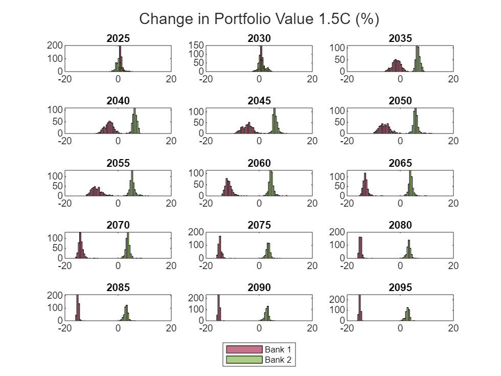
Create a histogram of the distribution of changes in valuation by year. In the 1.5C scenario, the greener Bank 2 distribution separates from Bank 1 much faster than in the 2C scenario.

scenario = "2C";
scenarioDataName = matlab.lang.makeValidName("percentChangeVal" + scenario);

figure;
t = tiledlayout(5,3);
for year = 2025:5:2095

    bank1Data = valChangeSummary(valChangeSummary.Snapshot == year & valChangeSummary.Bank == "Bank1",:);
    bank2Data = valChangeSummary(valChangeSummary.Snapshot == year & valChangeSummary.Bank == "Bank2",:);

    ax = nexttile;
    h1 = histogram(ax, bank1Data.(scenarioDataName));
    hold(ax, "on");
    h2 = histogram(ax, bank2Data.(scenarioDataName));
    h1.BinWidth = .5;
    h2.BinWidth = .5;
    titleString = string(year);
    title(ax, titleString);
    xlim(ax, [-20,20]);

    % Define colors for Bank 1 and Bank 2
    colorBank1 = [0.633, 0.078, 0.243];
    colorBank2 = [0.467, 0.675, 0.188];

    h1.FaceColor = colorBank1;
    h2.FaceColor = colorBank2;
    
end
leg = legend(["Bank 1", "Bank 2"]);
leg.Layout.Tile = "south";
title(t,"Change in Portfolio Value " + scenario +  " (%)");
fig = gcf;
currentPosition = get(fig, 'Position');
newHeight = currentPosition(4) * 2;
set(fig, 'Position', [currentPosition(1), currentPosition(2), currentPosition(3), newHeight]);

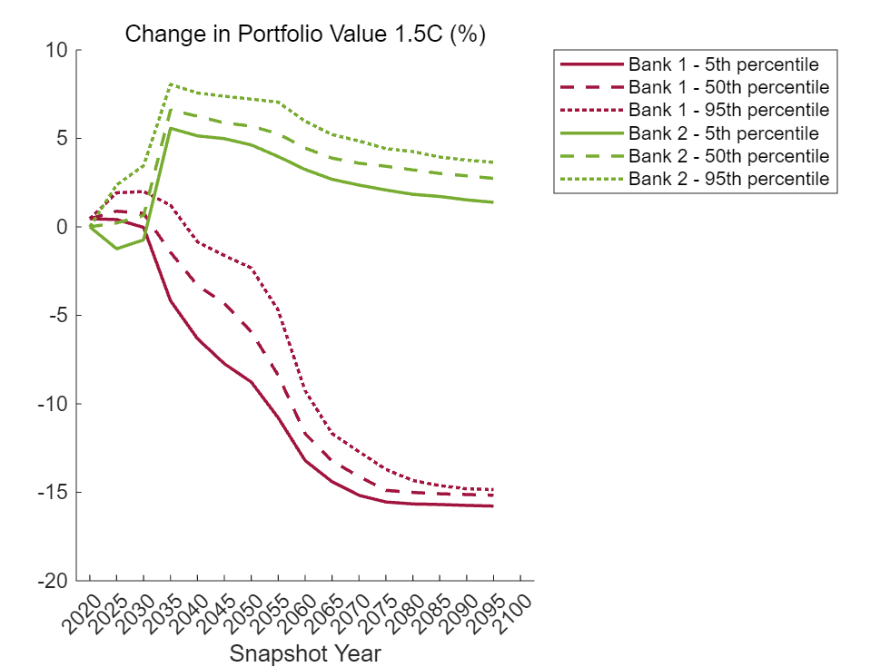
The following plots show the change in portfolio value by percentile in each snapshot. The losses for the Bank 1 are generally highest near the end of the horizon. The gains for Bank 2 are closer to the middle of the horizon. You can interpret the percentile values as a type of value-at-risk (VaR).

valChangePrctilesUnstack = unstack(valChangePrctiles, ...
    ["percentChangeVal1_5C_5","percentChangeVal1_5C_50","percentChangeVal1_5C_95","percentChangeVal2C_5","percentChangeVal2C_50","percentChangeVal2C_95"],"Bank");

x = valChangePrctilesUnstack.Snapshot;
scenario = "1.5C";
y = table2array(valChangePrctilesUnstack(:,contains(valChangePrctilesUnstack.Properties.VariableNames, matlab.lang.makeValidName("percentChangeVal" + scenario))));

figure;

% Plot Bank 1 lines
hold on;
plot(x, y(:,1), "-", 'LineWidth', 1.5, "Color", colorBank1, "DisplayName", "Bank 1 - 5th percentile");
plot(x, y(:,3), "--", 'LineWidth', 1.5, "Color", colorBank1, "DisplayName", "Bank 1 - 50th percentile");
plot(x, y(:,5), ":", 'LineWidth', 1.5, "Color", colorBank1, "DisplayName", "Bank 1 - 95th percentile");

% Plot Bank 2 lines
plot(x, y(:,2), "-", 'LineWidth', 1.5, "Color", colorBank2, "DisplayName", "Bank 2 - 5th percentile");
plot(x, y(:,4), "--", 'LineWidth', 1.5, "Color", colorBank2, "DisplayName", "Bank 2 - 50th percentile");
plot(x, y(:,6), ":", 'LineWidth', 1.5, "Color", colorBank2, "DisplayName", "Bank 2 - 95th percentile");

legend("Location","bestoutside");
xlabel("Snapshot Year");
title("Change in Portfolio Value " + scenario + " (%)", "FontWeight", "normal");
hold off;

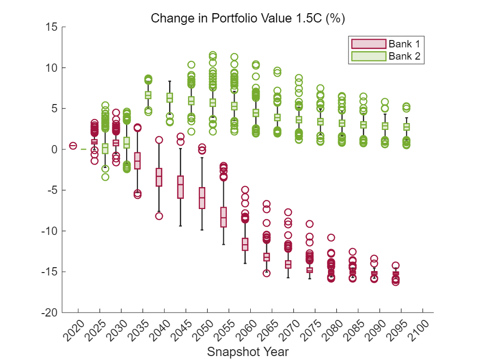
Figure contains an axes object. The axes object with title Change in Portfolio Value 1.5C (%), xlabel Snapshot Year contains 6 objects of type line. These objects represent Bank 1 - 5th percentile, Bank 1 - 50th percentile, Bank 1 - 95th percentile, Bank 2 - 5th percentile, Bank 2 - 50th percentile, Bank 2 - 95th percentile.

The box and whisker plots offer an alternative visualization. The Bank 1 pathways outperform Bank 2 in the short term, especially in the 2C scenario. The separation of distributions becomes clearer further into the future, and the separation occurs more quickly in the 1.5C scenario.

scenario = "1.5C";
scenarioDataName = matlab.lang.makeValidName("percentChangeVal" + scenario);

figure;
boxchart(valChangeSummary.Snapshot, valChangeSummary.(scenarioDataName), "GroupByColor", valChangeSummary.Bank);
colororder([colorBank1; colorBank2]);
xlabel("Snapshot Year");
title("Change in Portfolio Value " + scenario + " (%)", "FontWeight", "normal");
legend(["Bank 1", "Bank 2"]);

Figure contains an axes object. The axes object with title Change in Portfolio Value 1.5C (%), xlabel Snapshot Year contains 2 objects of type boxchart. These objects represent Bank 1, Bank 2.

Conclusion

The methodology used in this example provides a way to calculate the impact of climate scenarios on an obligor's PD. This example uses climate scenarios that have 400 simulations, which allows you to visualize a distribution of portfolio outcomes. The portfolio that is invested in green technologies performs better in the scenarios requiring a faster transition away from fossil fuels.

Methodology

Background

Monasterolo et al provide a methodology for performing a portfolio valuation that accounts for climate scenarios [1]. The methodology first computes a market share shock for different energy sectors based on the scenarios, and then converts this into a shock for the PD of each investment. By aggregating the shocks to the PD, you can calculate the change in value of the portfolio. For more information about this methodology, see [1].

Consider a financial actor endowed with a portfolio of investments through loan contracts. Each investment is represented as a distinct borrower, $j$ . Consider three time variables:

Let $t_{0}$ denote the time at which the portfolio valuation is taken.
Let $t^{*}$ denote the time at which a climate policy shock potentially occurs.
Let $t_{j}$ denote the maturity of borrower $j$ 's obligation.

In particular, for each borrower $j$ ,

$t_{0} < t^{*} < t_{j}$ .

Let $V_{j} (t_{0})$ denote the valuation of obligation $j$ at time $t_{0}$ . Then, the valuation of the portfolio at time $t_{0}$ , $V (t_{0})$ , is given by

$V (t_{0}) = \sum_{j} V_{j} (t_{0}) .$

Assume that the valuation of obligation $j$ is based on the expected value of the loan. For each obligor $j$ , consider the following:

Let $F_{j}$ denote the face value of the loan, already including the time-discounting factor.
Let $p_{j} (t_{0}) = p_{j} (t_{0}, t_{j})$ be the probability that the borrower defaults at time $t_{j}$ given the information available at time $t_{0}$ .
Let $r_{j}$ denote the recovery rate of the loan contract.

Then, assume

$V_{j} (t_{0}) = p_{j} (t_{0}) r_{j} F_{j} + (1 - p_{j} (t_{0})) F_{j} = F_{j} (1 - (1 - r_{j}) p_{j} (t_{0})) .$

Climate Policy Shocks

At time $t^{*}$ , the occurrence of a climate policy shock implies that the economy switches from a business-as-usual scenario characterized by no climate policy, $B$ , to a scenario, $P$ , where the market shares of some economic sectors are affected. Assume that this transition modifies the PD of the borrower $j$ through changes in the market share of the economic sector of $j$ . Let $Δ p_{j} (P, B)$ denote the change in default probability for obligor $j$ when going from scenario $B$ to scenario $P$ . The change in default probability implies a proportional change in the expected value of the loan:

$Δ V_{j} (t_{0}, P, B) = - F_{j} (1 - r_{j}) Δ p_{j} (P, B) .$

Next, assume $r_{j} = 0$ below.

Borrower's Default Conditions

Let $A_{j} (t, P, B)$ denote the total assets of borrower $j$ at time $t$ in scenario $P$ . Let $ξ_{j} (t^{*}, P, B)$ be the shock occurring at time $t^{*}$ associated with the shift from scenario $B$ to scenario $P$ . Let $η_{j} = η_{j} (t_{j})$ denote an exogenous stochastic shock hitting the asset side of the borrower at the maturity date $t_{j}$ . Then,

$A_{j} (t_{j}, P, B) = A_{j} (t_{0}) + ξ_{j} (t^{*}, P, B) + η_{j} .$

Assume that the borrower defaults at time $t_{j}$ if its net worth, defined as assets minus liabilities, at maturity becomes negative as a result of the two shocks. Let $E_{j} (t, P, B)$ denote the net worth at time $t$ in scenario $P$ . Note that $E_{j} (t_{0}, P, B) = E_{j} (t_{0})$ is independent of the climate scenarios. Let $L_{j}$ denote the value of obligor $j$ 's liabilities, which is assumed to be independent of time $t$ and the climate scenarios. Then, the default condition becomes

$E_{j} (t_{j}, P, B) = A_{j} (t_{j}, P, B) - L_{j} = A_{j} (t_{0}) + ξ_{j} (t^{*}, P, B) + η_{j} - L_{j} = E_{j} (t_{0}) + ξ_{j} (t^{*}, P, B) + η_{j} < 0 .$

You can rewrite the default condition as

$η_{j} < θ_{j} (P, B) = - (E_{j} (t_{0}) + ξ_{j} (t^{*}, P, B)) .$

When $P = B$ , there is no policy shock:

$η_{j} < θ_{j} (B, B) = - E_{j} (t_{0}) .$

Let $p_{j}$ be the probability density function of the idiosyncratic shock $η_{j}$ . Then,

$P {η_{j} < θ_{j} (P, B)} = \int_{- \infty}^{θ_{J} (P, B)} p_{j} (x) d x,$

which allows you to express the difference in probability as

$Δ p_{j} (P, B) = \int_{θ_{j} (B, B)}^{θ_{j} (P, B)} p_{j} (x) d x .$

Profitability and Shocks on Market Share

Assume that the policy shock impacts the obligor's balance sheet, and thus the expected value of the loan, via a change in the market share of the obligor's economic sector. Let $m_{S, R} (P, t^{*})$ denote the market share at time $t^{*}$ of sector $S$ in the region $R$ in scenario $P$ . Define $m_{S, R} (B, t^{*})$ similarly. Then the market share shock $u_{S, R} (P, B, t^{*})$ is defined as

$u_{S, R} (P, B, t^{*}) = \frac{m_{S, R} (P, t^{*}) - m_{S, R} (B, t^{*})}{m_{S, R} (B, t^{*})} .$

Let $χ$ denote the elasticity of profitability with respect to market share. A single value is chosen for all obligors. Assume that the relative change in net worth due to the change in scenarios is proportional to the relative market share shock:

$\frac{E_{j} (t_{j}, P, B) - E_{j} (t_{j}, B, B)}{E_{j} (t_{0})} = χ u_{S, R} (P, B, t^{*}) .$

Assume that $η_{j}$ is uniformly distributed with support width $δ_{j}$ and mean $μ_{j}$ . For $δ_{j}$ sufficiently large, you can express the difference in probability as

$Δ p_{j} (P, B) = \int_{θ_{j} (B, B)}^{θ_{j} (P, B)} p_{j} (x) = \frac{θ_{j} (P, B) - θ_{j} (B, B)}{δ_{j}} .$

Then,

$Δ p_{j} (P, B) = \frac{θ_{j} (P, B) - θ_{j} (B, B)}{δ_{j}} = \frac{- ξ_{j} (t^{*}, P, B)}{δ_{j}} = \frac{E_{j} (t_{j}, B, B) - E_{j} (t_{j}, P, B)}{δ_{j}} = - χ u_{S, R} (P, B, t^{*}) \frac{E_{j} (t_{0})}{δ_{j}} .$

The change in PD has been linked to the climate scenarios. However, you need to choose $δ_{j}$ and $χ$ appropriately. Assume that $χ = 1$ which you should view as a limitation because $χ$ could be chosen at the obligor level to reflect empirical data.

Before addressing $δ_{j}$ in more detail, consider the previous equation:

$Δ p_{j} (P, B) = - χ u_{S, R} (P, B, t *) \frac{E_{j} (t_{0})}{δ_{j}}$ .

The left hand side must be in the range [ $-$ 1,1]. However, the range in practice is actually much smaller. The climate scenarios in this example express a wide range of outcomes, which leads to very large shocks on the right side of the equation. As such, choose a sufficiently large $δ_{j}$ to move those shocks back into the expected range. You cap the shocks to keep them in a more reasonable range. In practice, an institution implementing this methodology decides what shock levels are consistent with their expectations and data.

Next, identify bounds for $δ_{j}$ . To compute $Δ p_{j} (P, B)$ as above, you need the interval of integration $[θ_{j} (B, B), θ_{j} (P, B)]$ to be contained in the support of the function $p_{j} (x)$ , which has been assumed to be $[μ_{j} - δ_{j} / 2, μ_{j} + δ_{j} / 2]$ . Since you have no view on the direction of the exogenous shock $η_{j}$ , assume that $μ_{j} = 0$ . It suffices for $δ_{j} / 2$ to be at least as large as $E_{j} (t_{0}) + a b s (ξ_{j} (t^{*}, P, B)) .$ The latter term is the absolute value of the shock $u_{S, R} (P, B, t^{*})$ times the starting book value $E_{j} (t_{0})$ . Choose $δ_{j}$ such that

$δ_{j} \geq 2 E_{j} (t_{0}) (1 + a b s (u_{S, R} (P, B, t^{*}))) .$

In practice, it is common to choose $δ_{j}$ to be equal to the right hand side.

Note that $δ_{j}$ implicitly depends on $P$ and $B$ and you can choose $δ_{j}$ uniformly across climate scenarios. As $δ_{j}$ reflects the size of the exogenous shocks, ensure that $δ_{j}$ does not depend on the choice of a particular climate scenario.

Finally, note that the quantity $E_{j} (t_{0}) / δ_{j}$ appearing in the expression for $Δ p_{j} (P, B)$ does not depend on $E_{j} (t_{0})$ when you choose $δ_{j}$ as above.

Local Functions

importClimateData

The following helper function reads in the downloaded Excel® climate data into a table based on the scenario, energy type, and region.

function climateData = importClimateData(scenario, energy, region)
    % Construct the path to the scenario folder
    scenarioFolder = fullfile(pwd, "MITUncertaintyData", scenario);

    % Find the file with the energy use data
    filePattern = fullfile(scenarioFolder, "*energy_use_" + energy + "*");
    fileStruct = dir(filePattern);
    file = fileStruct.name;
    filePath = fullfile(scenarioFolder, file);

    % Get the sheet names and find the index of the sheet that contains the region
    sheets = sheetnames(filePath);
    sheetIdx = contains(sheets, region);
    sheet = sheets(sheetIdx);

    % Set up the Import Options and import the data
    opts = spreadsheetImportOptions("NumVariables", 21);

    % Specify sheet and range
    opts.Sheet = sheet;
    opts.DataRange = "A2:U401";

    % Specify column names and types
    opts.VariableNames = ["Var1", "Var2", "Var3", "VarName4", "VarName5", "VarName6", "VarName7", "VarName8", "VarName9", "VarName10", "VarName11", "VarName12", "VarName13", "VarName14", "VarName15", "VarName16", "VarName17", "VarName18", "VarName19", "VarName20", "VarName21"];
    opts.SelectedVariableNames = ["VarName4", "VarName5", "VarName6", "VarName7", "VarName8", "VarName9", "VarName10", "VarName11", "VarName12", "VarName13", "VarName14", "VarName15", "VarName16", "VarName17", "VarName18", "VarName19", "VarName20", "VarName21"];
    opts.VariableTypes = ["char", "char", "char", "double", "double", "double", "double", "double", "double", "double", "double", "double", "double", "double", "double", "double", "double", "double", "double", "double", "double"];

    % Specify variable properties
    opts = setvaropts(opts, ["Var1", "Var2", "Var3"], "WhitespaceRule", "preserve");
    opts = setvaropts(opts, ["Var1", "Var2", "Var3"], "EmptyFieldRule", "auto");
    opts = setvaropts(opts, ["VarName4", "VarName5", "VarName6", "VarName7", "VarName8", "VarName9", "VarName10", "VarName11", "VarName12", "VarName13", "VarName14", "VarName15", "VarName16", "VarName17", "VarName18", "VarName19", "VarName20", "VarName21"], "FillValue", 0);

    % Import the data
    climateData = readtable(filePath, opts, "UseExcel", false);

    clear opts

    % Reshape and format the data
    climateData = stack(climateData,2:18,"NewDataVariableName","Energy Use","IndexVariableName","Year");
    climateData.Year = renamecats(climateData.Year,["VarName5","VarName6","VarName7","VarName8","VarName9","VarName10","VarName11","VarName12","VarName13","VarName14","VarName15","VarName16","VarName17","VarName18","VarName19","VarName20","VarName21"], ...
        ["2020", "2025", "2030", "2035", "2040", "2045", "2050", "2055", "2060", "2065", "2070", "2075", "2080", "2085", "2090", "2095", "2100"]);

    dataHeight = height(climateData);
    climateData = renamevars(climateData,"VarName4","Simulation");
    climateData.Scenario = categorical(repmat(scenario,[dataHeight 1]));
    climateData.Region = categorical(repmat(region,[dataHeight 1]));
    climateData.Energy = categorical(repmat(energy,[dataHeight 1]));
end

References

[1] Monasterolo, I., Zheng, Jiani I., and S. Battiston. "Climate Transition Risk and Development Finance: A Carbon Risk Assessment of China's Overseas Energy Portfolios." China and World Economy. 26, 6(116–142), 2018. Available at: https://onlinelibrary.wiley.com/doi/epdf/10.1111/cwe.12264.