loopmargin

(Not recommended) Stability margin analysis of LTI and Simulink feedback loops

loopmargin is not recommended. Use diskmargin or allmargin instead. For more information, see Version History.

Syntax

[cm,dm,mm] = loopmargin(L)
[m1,...,mn] = loopmargin(L,MFLAG)
[cmi,dmi,mmi,cmo,dmo,mmo,mmio] = loopmargin(P,C)
[m1,...,mn] = loopmargin(P,C,MFLAG)
[cm,dm,mm] = loopmargin(Model,Blocks,Ports)
[cm,dm,mm,info] = loopmargin(Model,Blocks,Ports,OP)
[m1,...,mn,info] = loopmargin(Model,Blocks,Ports,MFLAG)
[m1,...,mn,info] = loopmargin(Model,Blocks,Ports,OP,MFLAG)


Description

[cm,dm,mm] = loopmargin(L) analyzes the multivariable feedback loop consisting of the loop transfer matrix L (size N-by-N) in negative feedback with an N-by-N identity matrix.

cm, or classical gain and phase margins, is an N-by-1 structure corresponding to loop-at-a-time gain and phase margins for each channel. L is an LTI model. Use -L to specify positive feedback.

dm is an N-by-1 structure corresponding to loop-at-a-time disk gain and phase margins for each channel. The disk margin for the i-th feedback channel defines a circular region centered on the negative real axis at the average GainMargin (GM), e.g. , (GM_low+GM_high)/2, such that L(i,i) does not enter that region. Gain and phase disk margin bounds are derived from the radius of the circle, calculated based on the balanced sensitivity function.

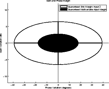
mm, the multiloop disk margin, is a structure. mm describes how much independent and concurrent gain and phase variation can occur independently in each feedback channel while maintaining stability of the closed-loop system. Note that mm is a single structure, independent of the number of channels. This is because variations in all channels are considered simultaneously. As in the case for disk margin, the guaranteed bounds are calculated based on a balanced sensitivity function.

[m1,...,mn] = loopmargin(L,MFLAG) returns a subset of the margins, specified by the character vector MFLAG. This optional argument may be any combination, in any order, of the 3 characters 'c', 'd' and 'm'. For example, [m1,m2] = loopmargin(L,'m,c') returns the multi-loop disk margin ('m') in m1, and the classical margins ('c') in m2. Use 'd' to specify the disk margin.

[cmi,dmi,mmi,cmo,dmo,mmo,mmio] = loopmargin(P,C) analyzes the multivariable feedback loop consisting of the controller C in negative feedback with the plant, P. C should only be the compensator in the feedback path, without reference channels, if it is a two-degree-of-freedom (2-dof) architecture. That is, if the closed-loop system has a 2-dof architecture the reference channel of the controller should be eliminated, resulting in a 1-dof architecture, as shown.

cmi,dmi and mmi structures correspond to the classical loop-at-a-time gain and phase margins, disk margins and multiloop channel margins at the plant input respectively. The structures cmo, dmo and mmo have the same fields as described for cmi, dmi and mmi though they correspond to the plant outputs. mmio, or multi-input/multi-output margins, is a structure corresponding to simultaneous, independent, variations in all the individual input and output channels of the feedback loops. mmio has the same fields as mmi and mmo.

[m1,...,mn] = loopmargin(P,C,MFLAG) returns a subset of the margins, specified by MFLAG. This optional argument may be any combination, in any order, of the 7 character pairs 'ci', 'di', 'mi', 'co', 'do, 'mo', and 'mm'. For example,[m1,m2,m3] = loopmargin(P,C,'mo,ci,mm') returns the multi-loop disk margin at the plant output ('mo') in m1, the classical margins at the plant input ('ci') in m2, and the multi-loop disk margins for simultaneous, independent variations in all input and output channels ('mm') in m3.

Usage with Simulink

[cm,dm,mm] = loopmargin(Model,Blocks,Ports) does a multi-loop stability margin analysis using Simulink^® Control Design™ software. Model specifies the name of the Simulink diagram for analysis. The margin analysis points are defined at the output ports (Ports) of blocks (Blocks) within the model. Blocks is a cell array of full block path names and Ports is a vector of the same dimension as Blocks. If all Blocks have a single output port, then Ports would be a vector of ones with the same length as Blocks.

Three types of stability margins are computed: loop-at-a-time classical gain and phase margins (cm), loop-at-a-time disk margins (dm) and a multi-loop disk margin (mm).

[cm,dm,mm] = loopmargin(Model,Blocks,Ports,OP) uses the operating point object OP to create linearized systems from the Simulink Model.

[cm,dm,mm,info] = loopmargin(Model,Blocks,Ports,OP) returns info in addition to the margins. info is a structure with fields OperatingPoint, LinearizationIO and SignalNames corresponding to the analysis.

[m1,...,mn,info] = loopmargin(Model,Blocks,Ports,MFLAG) and [m1,...,mn,info] = loopmargin(Model,Blocks,Ports,OP,MFLAG) return a subset of the margins, specified by the character vector MFLAG. This optional argument may be any combination, in any order, of the 3 characters 'c', 'd' and 'm'. For example, [m1,m2] = loopmargin(Model,Blocks,Ports,'m,c') returns the multi-loop disk margin ('m') in m1, and the classical margins ('c') in m2. Use 'd' to specify the disk margin.

Basic Syntax

[cm,dm,mm] = loopmargin(L) cm is calculated using the allmargin command and has the same fields as allmargin. The output cm is an N-by-1 structure of classical gain and phase margins for each feedback channel with all other loops closed. cm has the following fields:

Field	Description
GMFrequency	All –180 deg crossover frequencies (in radians-per-second)
GainMargin	Corresponding gain margins (GM = 1/L where L is the gain at crossover)
PhaseMargin	Corresponding phase margins (in degrees)
PMFrequency	All 0 dB crossover frequencies (in radians-per-second)
DelayMargin	Delay margins (in seconds for continuous-time systems, and multiples of the sample time for discrete-time systems)
Stable	1 if nominal closed loop is stable, 0 otherwise. If L is a frd or ufrd object, the Stable flag is set to NaN.

dm, or Disk Margin, is an N-by-1 structure of disk margins for each feedback channel with all other loops closed. dm has the following fields:

Field	Description
GainMargin	Smallest gain variation (GM) such that a disk centered at the point –(GM(1) + GM(2))/2 just touches the Nyquist plot of the loop transfer function.
PhaseMargin	Smallest phase variation, in degrees, corresponding to the disk described in the GainMargin field.
Frequency	Frequency with the weakest disk margin, in rad/TimeUnit, where TimeUnit is the TimeUnit property of L. For frd models, loopmargin computes margins at all the frequency points in the model, and returns the frequency with the weakest margin of these values.

mm is a structure with the following fields.

Field	Description
GainMargin	Guaranteed bound on simultaneous, independent, gain variations allowed in all plant channels.
PhaseMargin	Guaranteed bound on simultaneous, independent, phase variations allowed in all plant channels (degrees).
Frequency	Frequency with the weakest disk margin, in rad/TimeUnit, where TimeUnit is the TimeUnit property of L. For frd models, loopmargin computes margins at all the frequency points in the model, and returns the frequency with the weakest margin of these values.

Relationship Between Disk Margin and Gain and Phase Margins

The disk margin is based on a multiplicative uncertainty model in which the loop gain L of each loop channel becomes

$$L\to L\frac{1+\Delta /2}{1-\Delta /2},\left|\Delta \right|<\alpha .$$

where Δ is complex. The uncertainty size α is the disk margin. The uncertain quantity (1 + Δ)/(1 – Δ) has a gain component and a phase component. Thus, enforcing a disk margin α also enforces minimum gain and phase margins given by

$$\begin{array}{l}GM=\frac{1+\alpha }{1-\alpha },\\ PM=2\arctan \left(\alpha \right),\end{array}$$

with GM in absolute units and PM in degrees. The gain and phase margins are therefore related by

$$GM=\frac{1+\tan \left(PM/2\right)}{1-\tan \left(PM/2\right)}.$$

When you specify independent gain and phase margins for tuning, the software chooses the smallest α that enforces both values, which is

$$\alpha =2\left(\max \left[\frac{GM-1}{GM+1},\tan \left(PM/2\right)\right]\right).$$

Note that GM and PM are not the same as the classical gain and phase margins. Rather, they provide stronger guarantees of stability, because both of the following can occur at the same time without loss of stability:

• The loop gain can increase or decrease by a factor of GM, and

• The loop phase can increase or decrease by PM degrees.

By contrast, the classical gain and phase margins consider only gain variations or phase variations at a single frequency, the crossover frequency.

Examples

MIMO Loop-at-a-Time Margins

This example shows how to compute loop-at-a-time margins (gain, phase, and/or distance to –1), and also illustrates that such margins can be inaccurate measures of multivariable robustness margins. Margins of individual loops can be very sensitive to small perturbations within other loops.

Consider the nominal closed-loop system of the following illustration.

G and K are 2-by-2 (MIMO) systems, given by:

$$G=\frac{1}{s^2+{\alpha }^2}\left[\begin{array}{cc}{s}^2-{\alpha }^2& \alpha \left(s+1\right)\\ -\alpha \left(s+1\right)& s^2-{\alpha }^2\end{array}\right],K=\left[\begin{array}{cc}1& -2\\ 0& 1\end{array}\right].$$

Set α = 10, construct G in state-space form, and compute the loop margins.

a = [0 10;-10 0]; 
b = eye(2); 
c = [1 8;-10 1]; 
d = zeros(2,2); 
G = ss(a,b,c,d); 
K = [1 -2;0 1]; 
[cmi,dmi,mmi,cmo,dmo,mmo,mmio] = loopmargin(G,K);

First consider the margins at the input to the plant. The first input channel has infinite gain margin and 90 degrees of phase margin based on the results from the loopmargin command, cmi(1).

cmi(1)

ans = struct with fields:
     GainMargin: [1x0 double]
    GMFrequency: [1x0 double]
    PhaseMargin: 90
    PMFrequency: 21
    DelayMargin: 0.0748
    DMFrequency: 21
         Stable: 1

The disk margin analysis, dmi, of the first channel provides similar results.

dmi(1)

ans = struct with fields:
     GainMargin: [0 Inf]
    PhaseMargin: [-90 90]
      Frequency: 0

The second input channel has a gain margin of 2.105 and infinite phase margin based on the single-loop analysis, cmi(2).

cmi(2)

ans = struct with fields:
     GainMargin: 2.1053
    GMFrequency: 0
    PhaseMargin: [1x0 double]
    PMFrequency: [1x0 double]
    DelayMargin: [1x0 double]
    DMFrequency: [1x0 double]
         Stable: 1

The disk margin analysis, dmi(2), which allows for simultaneous gain and phase variations a loop-at-a-time results in maximum gain margin variations of 0.475 and 2.105 and phase margin variations of +/- 39.18 degs.

dmi(2)

ans = struct with fields:
     GainMargin: [0.4750 2.1053]
    PhaseMargin: [-39.1846 39.1846]
      Frequency: 0

The multiple margin analysis of the plant inputs corresponds to allowing simultaneous, independent gain and phase margin variations in each channel. Allowing independent variation of the input channels further reduces the tolerance of the closed-loop system to variations at the input to the plant. The multivariable margin analysis, mmi, leads to a maximum allowable gain margin variation of 0.728 and 1.373 and phase margin variations of +/- 17.87 deg. Hence even though the first channel had infinite gain margin and 90 degrees of phase margin, allowing variation in both input channels leads to a factor of two reduction in the gain and phase margin.

mmi

mmi = struct with fields:
     GainMargin: [0.7288 1.3721]
    PhaseMargin: [-17.8304 17.8304]
      Frequency: 0

The guaranteed region of phase and gain variations for the closed-loop system can be illustrated graphically. The disk margin analysis, dmi(2), indicates the closed-loop system will remain stable for simultaneous gain variations of 0.475 and 2.105 (± 6.465 dB) and phase margin variations of ± 39.18 deg in the second input channel. This is denoted by the region associated with the large ellipse in the following figure. The multivariable margin analysis at the input to the plant, mmi, indicates that the closed-loop system will be stable for independent, simultaneous, gain margin variation up to 0.728 and 1.373 (±2.753 dB) and phase margin variations up to ± 17.87 deg (the dark ellipse region) in both input channels.

The output channels have single-loop margins of infinite gain and 90 deg phase variation. The output multivariable margin analysis, mmo, leads to a maximum allowable gain margin variation of 0.607 and 1.649 and phase margin variations of +/- 27.53 degs. Hence even though both output channels had infinite gain margin and 90 degrees of phase margin, simultaneous variations in both channels significantly reduce the margins at the plant outputs.

mmo

mmo = struct with fields:
     GainMargin: [0.6070 1.6474]
    PhaseMargin: [-27.4826 27.4826]
      Frequency: 0.2663

The margins when all the input and output channels are allowed to vary independently are in the output mmio. For this system, this output shows that the allowable gain margin variations are 0.827 and 1.210 and allowable phase margin variations are +/- 10.84 deg.

mmio

mmio = struct with fields:
     GainMargin: [0.8270 1.2092]
    PhaseMargin: [-10.8190 10.8190]
      Frequency: 0

Algorithms

Two well-known loop robustness measures are based on the sensitivity function S=(I–L)^–1 and the complementary sensitivity function T=L(I–L)^–1 where L is the loop gain matrix associated with the input or output loops broken simultaneously. In the following figure, S is the transfer matrix from summing junction input u to summing junction output e. T is the transfer matrix from u to y. If signals e and y are summed, the transfer matrix from u to e+y is given by (I+L)· (I–L)^–1, the balanced sensitivity function. It can be shown (Dailey, 1991, Blight, Daily and Gangass, 1994) that each broken-loop gain can be perturbed by the complex gain (1+Δ)(1–Δ) where |Δ|<1/µ(S+T) or |Δ|<1/σ_max(S+T) at each frequency without causing instability at that frequency. The peak value of µ(S+T) or σ_max(S+T) gives a robustness guarantee for all frequencies, and for µ(S+T) the guarantee is nonconservative (Blight, Daily and Gangass, 1994).

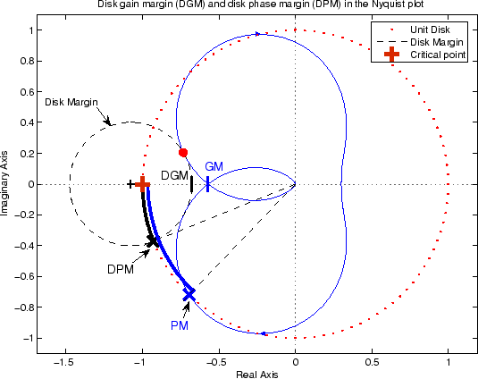
This figure shows a comparison of a disk margin analysis with the classical notations of gain and phase margins.

The Nyquist plot is of the loop transfer function L(s)

$$L(s)=\frac{\frac{s}{30}+1}{(s+1)(s^2+1.6s+16)}$$

• The Nyquist plot of L corresponds to the blue line.

• The unit disk corresponds to the dotted red line.

• GM and PM indicate the location of the classical gain and phase margins for the system L.

• DGM and DPM correspond to the disk gain and phase margins. The disk margins provide a lower bound on classical gain and phase margins.

• The disk margin circle corresponds to the dashed black line. The disk margin corresponds to the largest disk centered at (GMD + 1/GMD)/2 that just touches the loop transfer function L. This location is indicated by the red dot.

The disk margin and multiple channel margins calculation involve the balanced sensitivity function S+T. For a given peak value of µ(S+T), any simultaneous phase and gain variations applied to each loop independently will not destabilize the system if the perturbations remain inside the corresponding circle or disk. This corresponds to the disk margin calculation to find dmi and dmo.

Similarly, the multiple channel margins calculation involves the balanced sensitivity function S+T. Instead of calculating µ(S+T) a single loop at a time, all the channels are included in the analysis. A µ-analysis problem is formulated with each channel perturbed by an independent, complex perturbation. The peak µ(S+T) value guarantees that any simultaneous, independent phase and gain variations applied to each loop simultaneously will not destabilize the system if they remain inside the corresponding circle or disk of size µ(S+T).

For frequency-response data (frd) models, loopmargin uses the techniques of μ-analysis to compute the disk margin at each frequency point in the model, and returns the weakest margin of these values. For all other models, the μ-analysis computation identifies the frequency with the weakest margin.

References

Barrett, M.F., Conservatism with robustness tests for linear feedback control systems, Ph.D. Thesis, Control Science and Dynamical Systems, University of Minnesota, 1980.

Blight, J.D., R.L. Dailey, and D. Gangsass, “Practical control law design for aircraft using multivariable techniques,” International Journal of Control, Vol. 59, No. 1, 1994, pp. 93-137.

Bates, D., and I. Postlethwaite, “Robust Multivariable Control of Aerospace Systems,” Delft University Press, Delft, The Netherlands, ISBN: 90-407-2317-6, 2002.

Version History

Introduced before R2006a

R2018b: loopmargin is not recommended

To compute disk-based stability margins of SISO and MIMO systems, use diskmargin. For loop-at-a-time classical gain margins, use allmargin. For stability margin analysis of feedback loops modeled in Simulink, first linearize the model and then use diskmargin. For more information, see Stability Margins of a Simulink Model.

diskmargin, introduced in R2018b, has improved numeric stability and more reliable results relative to loopmargin. The new command also includes an option for varying the skew of the disk for better margin estimates. For more information, see diskmargin.

Update Code

To update your code to use diskmargin or allmargin:

Old code	New code
[CM,DM,MM] = loopmargin(L)	[DM,MM] = diskmargin(L) returns the disk margins of each feedback channel with all other loops closed in the structure DM, and the multiloop disk margin in the structure MM. S = allmargin(L) returns the classical loop-at-a-time gain and phase margins returned by loopmargin as CM. The margins are organized differently in the structure S. For more information, enter help allmargin at the MATLAB® command prompt.
[CMI,DMI,MMI,CMO,DMO,MMO,MMIO] = loopmargin(P,C)	MMIO = diskmargin(L) All the multiloop disk margins returned by loopmargin are in the structure MMIO.
[cm,dm,mm] = loopmargin(Model,Blocks,Ports)	First linearize the Simulink model and then use diskmargin or allmargin. For more information, see Stability Margins of a Simulink Model.