Find Zeros, Poles, and Gains for CTLE from Transfer Function

This example shows how to use the CTLE Fitter app to configure a CTLE block from SerDes Toolbox™ in the SerDes Designer app or in Simulink®. You can use the CTLE Fitter app to fit zeros, poles, and gains from a transfer function to create a GPZ Matrix and then export to your workspace. The CTLE Fitter app finds the GPZ Matrix by performing a fit comparison to a transfer function using the rational (RF Toolbox) function from RF Toolbox™.

Using CTLE Fitter App

You can open the CTLE Fitter app from SerDes Toolbox using any of the three workflows:

• From the CTLE block in the SerDes Designer app.

• From the CTLE block in the Simulink model.

• From the MATLAB® command window in the standalone mode.

Configure CTLE Block in SerDes Designer App

This workflow creates a variable representing a GPZ Matrix in the base workspace that is referenced by the CTLE block GPZ properties field in the SerDes Designer App. The steps are:

• Add a CTLE block and click the button Launch CTLE Fitter App.

• Import a CTLE frequency response. There can also be multiple responses in your data file.

• Adjust preprocess options for your transfer function data.

• Configure parameters of the rational function from RF Toolbox to optimize the fit to the transfer function.

• Visualize the fit response within the CTLE Fitter app using plots provided for magnitude response and pulse response.

• Close the CTLE Fitter app and continue with your session in the SerDes Designer app.

Simulink SerDes Model with CTLE block

This workflow creates a variable representing a GPZ Matrix in the model workspace and references this in the CTLE block mask GPZ field. The steps are:

• Open the CTLE block mask and click the button Launch CTLE Fitter App.

• Import a CTLE frequency response.

• Adjust preprocess options for your transfer function data.

• Configure parameters of the rational function from RF Toolbox to optimize the fit to the transfer function.

• Visualize the fit response within the CTLE Fitter app using plots provided for magnitude response and pulse response.

• Close the CTLE Fitter app and continue with your session in Simulink.

Standalone Mode

This workflow creates a variable in the base workspace representing a GPZ Matrix. The steps are:

• Launch the app with the MATLAB command ctlefitter.

• Import a CTLE frequency response.

• Adjust preprocess options for your transfer function data.

• Configure parameters of the rational function from RF Toolbox to optimize the fit to the transfer function.

• Visualize the fit response within the CTLE Fitter app using plots provided for magnitude response and pulse response.

• You have the option to both export a script and save a GPZ Matrix to the base workspace.

• Close the CTLE Fitter app and continue with your session in MATLAB

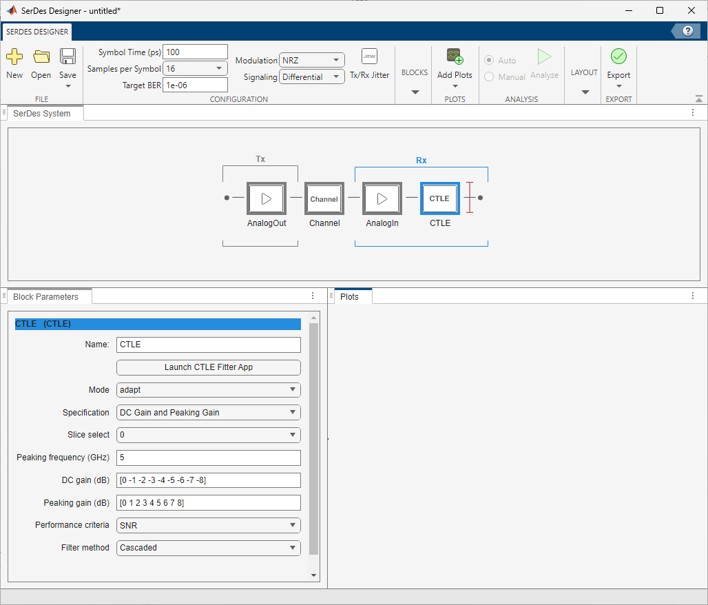
Configure CTLE Block in the SerDes Designer App

Launch the SerDes Designer app. Place a CTLE block after the analog model of the receiver. Then in the Block Parameters section, you can click on the button to launch the CTLE Fitter App.

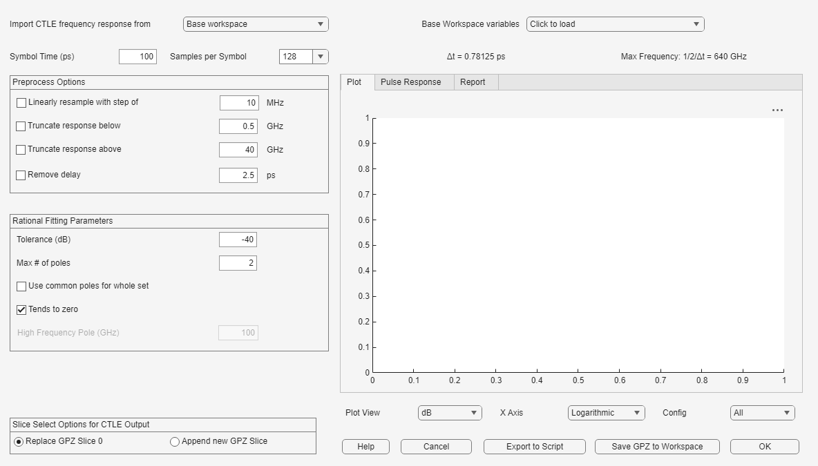
Import One or More CTLE Frequency Responses

The app will open with some default values shown. Follow these steps to import a file containing one or more CTLE frequency responses:

• Click on the dropdown menu "Import CTLE frequency response from" and select the "CSV" option

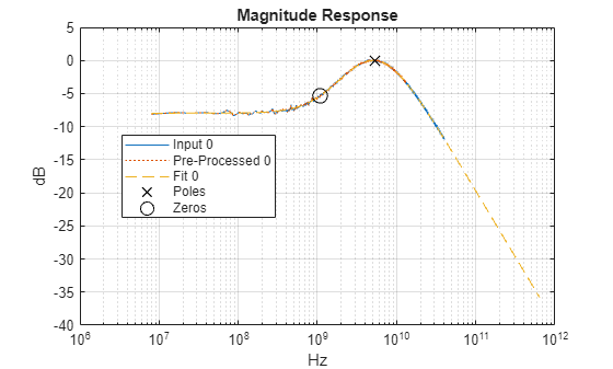
• Click the Browse button to open a .csv file containing a transfer function. Note: You can use the file attached to this example "CTLEdefault1RealImag.csv" to explore the features of the ctlefitter app. In the screenshots below, this file has been placed in the folder "D:\data" but may be in a different location on your system.

• You will see the app loads the file and automatically updates the figure shown on the Plot tab:

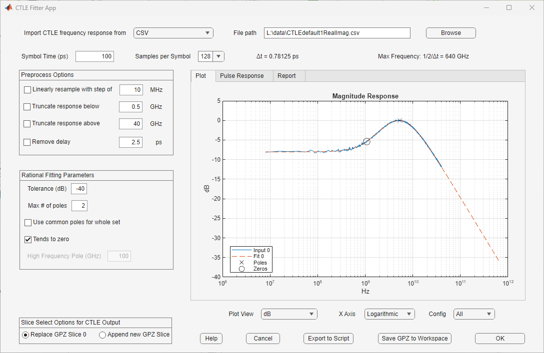
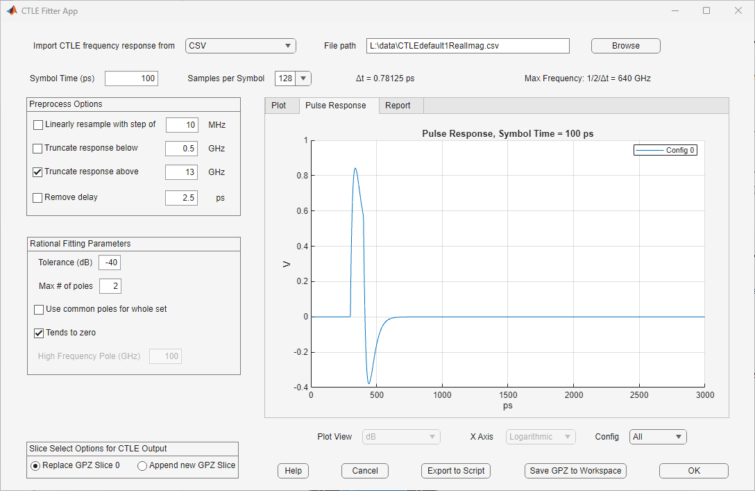
Adjust Preprocess Options

In the app, you can see many Preprocess Options are available. For example it is possible to truncate the data set from the transfer function used by the Fit. In the screenshot below you can see this is set to a cutoff frequency of 13 GHz:

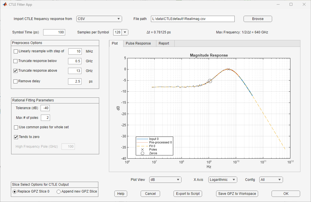
You can also adjust:

• Linearly resample with step size in MHz

• Truncate response below a specified frequency in GHz

• Truncate response above a specified frequency in GHz

• Remove delay in picoseconds

Configure Rational Fitting Parameters

You can configure the way the MATLAB function rational determines a fit by adjusting the following:

• Error tolerance (dB)

• Maximum number of poles

• Use common poles for whole set

• Enable or disable "tends to zero"

These parameters are explained in the documentation for the MATLAB function rational, which is part of the RF Toolbox.

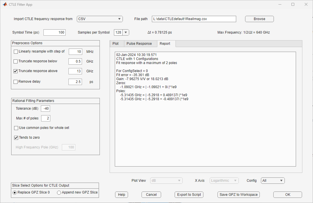
Report on Rational Fit Results

You can view the statistical parameters of the fit reported by the MATLAB function rational on the "Report" tab:

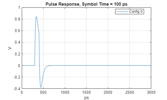
Pulse Response

You can view the pulse response on the Pulse Response tab:

Export a GPZ Matrix for CTLE Block

You can export the GPZ Matrix to the Workspace by clicking on the button "Save GPZ to Workspace."

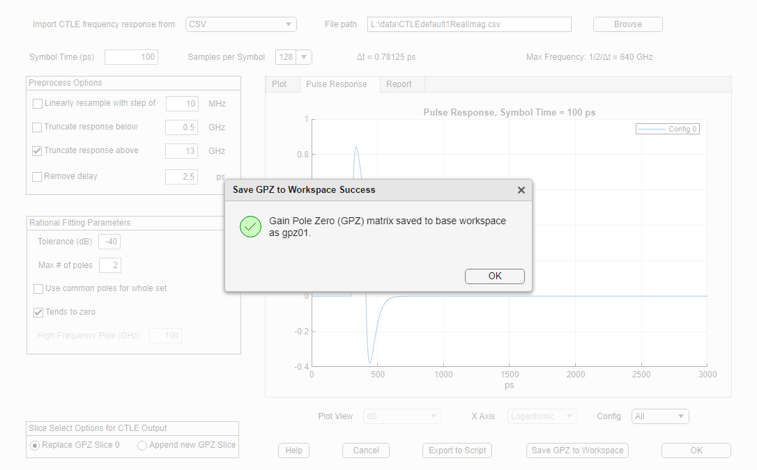
Note: If you have previously exported a GPZ Matrix, the name will automatically increment. For example, gpz01 is created in the figure below, but if gpz01 already exists in the workspace it would be automatically named gpz02 and added to your workspace.

Export Script from CTLE Fitter App to Base Workspace

You can also export a script from the ctlefitter app to the base workspace by clicking on the button "Export to Script" and you can see example output below.

Note: The script contents you see may differ from the example below- depending on the data file being analyzed and your specific CTLE configuration options.

%Read in file:
fn = 'CTLEdefault1RealImag.csv';
[f,H]=ctlefit.readcsv(fn);

SymbolTime = 1e-10;

%Initialize ctleit object
obj = ctlefit(...
    'f',f,...
    'H',H,...
    'SampleInterval',7.8125e-13,...
    'MaxNumberOfPoles',2,...
    'ErrorTolerance',-40,...
    'TendsToZero',1,...
    'UseCommonPoles',0,...
    'PaddedPole',1e+11);

%Preprocess transfer function waveform
df = 1e+07;
%resample(obj,df);
fcut1 = 5e+08;
%truncateBelow(obj,fcut1);
fcut2 = 1.3e+10;
truncateAbove(obj,fcut2);
delay = 2.5e-12;
%removeDelay(obj,delay);

%Get GPZ matrix
gpz = obj.GPZ;

%Visualize and create report
%TFView (Transfer function view) can be 'dB', 'Phase', 'Real/Imag',
%'Phase Delay', 'Group Delay'.
TFView = 'dB';
%ConfigSelect (CTLE Configuration Select) can be - 'All', 'Worst fit', 0 to
%N-1, where N is the number of configurations.
ConfigSelect = 'All';
%AxisStyle can be 'semilogx', 'plot', 'semilogy' or 'loglog'.
AxisStyle = 'semilogx';
figure,
plot(obj,TFView,ConfigSelect,AxisStyle)

figure,
plotPulse(obj,ConfigSelect,SymbolTime)

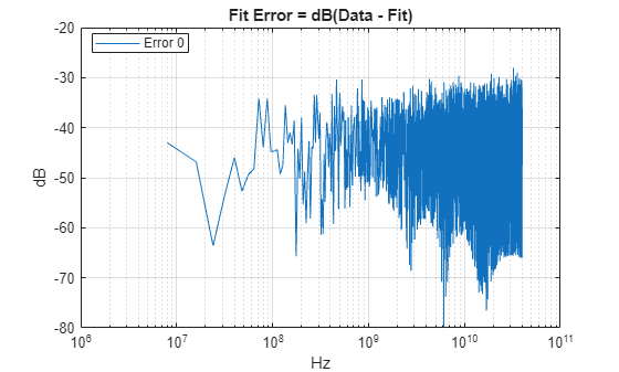
figure,
plotError(obj,ConfigSelect)

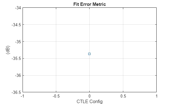
figure,
plotFitMetric(obj)

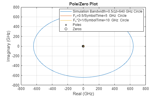
figure,
plotPoleZero(obj,ConfigSelect,SymbolTime)

report(obj,'All');

15-Jul-2022 12:36:23.11
CTLE with 1 Configurations
Fit response with a maximum of 2 poles
 
For ConfigSelect = 0
Fit error = -35.361 dB
Gain: -7.96275 V/V or 18.0213 dB
Zeros:
    -1.09021 GHz = | -1.09021 + 0i |*1e9
Poles:
    -5.31435 GHz = | -5.2918 + 0.489137i |*1e9
    -5.31435 GHz = | -5.2918 + -0.489137i |*1e9

Simulink SerDes Model with CTLE block

You can configure a Simulink SerDes Model with a CTLE block by opening the CTLE block parameters and click the “Launch CTLE Fitter App" button. You can follow the same steps outlined above in the section Configure CTLE Block in the SerDes Designer App to configure the CTLE Fitter app and export a GPZ Matrix for use in a CTLE block.

In the Block Parameters of the CTLE, you can click the button to launch the ctlefitter app:

After you close the ctlefitter app, you will see the CTLE block is automatically configured to use the GPZ Matrix it created:

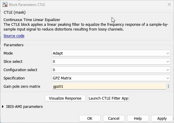
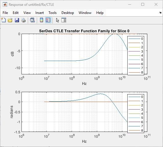
You can confirm the transfer function represented by the GPZ Matrix has a reasonable magnitude and phase response by clicking on "Visualize Response" button. These plots are also available in the SerDes Designer app workflow, and further detailed plots are provided as part of the exported script template.

Standalone Mode

Open the CTLE fitter app from the MATLAB command window:

ctlefitter;

You can follow the same steps outlined above in the section Configure CTLE Block in the SerDes Designer App to configure the CTLE Fitter app and export a GPZ Matrix to the base workspace in your MATLAB session.

Once you browse to and open a file containing one or more CTLE filter responses, you will see the app automatically updates the figure shown on the Plot tab: