findpeaks

Find local maxima

Syntax

pks = findpeaks(y)

[pks,locs] = findpeaks(y)

[pks,locs,w,p] = findpeaks(y)

[___] = findpeaks(y,x)

[___] = findpeaks(y,Fs)

[___] = findpeaks(___,Name=Value)

findpeaks(___)

Description

pks = findpeaks(y) returns a vector with the local maxima (peaks) of the input signal vector, y. A local peak is a data sample that is either larger than its two neighboring samples or is equal to an Inf value. The function outputs the peaks in order of occurrence and excludes non-Inf signal endpoints. If a peak is flat, the function returns only the point with the lowest index.

[pks,locs] = findpeaks(y) additionally returns the indices at which the peaks occur.

[pks,locs,w,p] = findpeaks(y) also returns the widths of the peaks as the vector w and the prominences of the peaks as the vector p.

[___] = findpeaks(y,x) specifies x as the location vector and returns any of the output arguments from previous syntaxes. locs and w are expressed in terms of x.

[___] = findpeaks(y,Fs) specifies the sample rate, Fs, of the data. The function assumes that the first sample of y is taken at time zero. locs and w are converted to time units.

[___] = findpeaks(___,Name=Value) specifies options using name-value arguments in addition to any of the input arguments in previous syntaxes.

findpeaks(___) without output arguments plots the signal and overlays the peak values.

Examples

Find Peaks in Vector

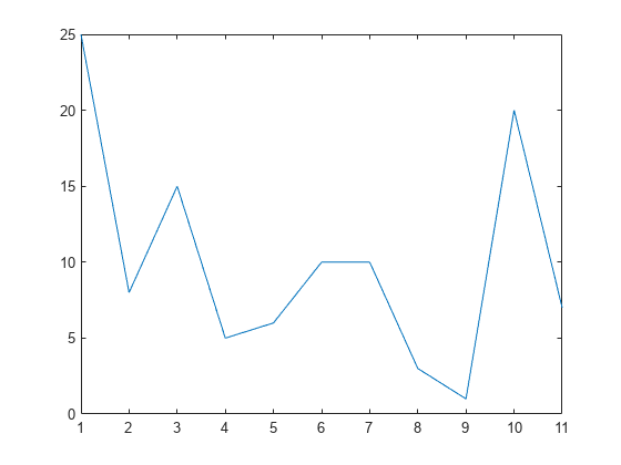
Define a vector with three peaks.

data = [25 8 15 5 6 10 10 3 1 20 7];

Find the local maxima. The findpeaks function returns peaks in order of occurrence. The function does not include the endpoints of data in the peak finding because there is no left or right neighbor to compare the endpoints with.

pks = findpeaks(data)

pks = 1×3

    15    10    20

Use findpeaks without output arguments to display the peaks. For the flat peak, the function highlights only the point with the lowest index.

findpeaks(data)

Find Peaks and Their Locations

Create a signal that consists of a sum of Gaussian curves. Specify the position, height, and width of each curve.

x = linspace(0,1,1000);

Pos = [1 2 3 5 7 8]'/10;
Hgt = [3 4 4 2 2 3]';
Wdt = [2 6 3 3 4 6]'/100;

y = sum(Hgt.*(exp(-((x-Pos)./Wdt).^2)),1);

Use findpeaks with default settings to find the peaks of the signal and their locations.

[pks,locs] = findpeaks(y,x);

Plot the peaks using findpeaks. Label each peak.

findpeaks(y,x)
text(locs+.02,pks,num2str((1:numel(pks))'))

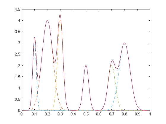
Sort the peaks from tallest to shortest.

[psor,lsor] = findpeaks(y,x,SortStr="descend");
findpeaks(y,x)
text(lsor+.02,psor,num2str((1:numel(psor))'))

Peak Prominences

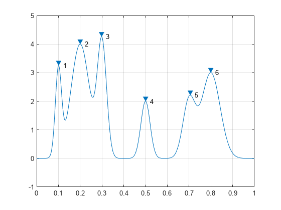
Create a signal that consists of a sum of Gaussian curves riding on a full period of a cosine. Specify the location, height, and width of each curve.

x = linspace(0,1,1000);

base = 4*cos(2*pi*x);

Pos = [1 2 3 5 7 8]'/10;
Hgt = [3 7 5 5 4 5]';
Wdt = [1 3 3 4 2 3]'/100;

y = sum(Hgt.*(exp(-((x-Pos)./Wdt).^2)),1) + base;

Use findpeaks to locate and plot the peaks that have a prominence of at least 4. Only the highest and lowest peaks satisfy the minimum prominence condition.

[~,locs4,~,proms4] = findpeaks(y,x,MinPeakProminence=4)

locs4 = 1×2

    0.1982    0.4995

proms4 = 1×2

    5.5773    4.4171

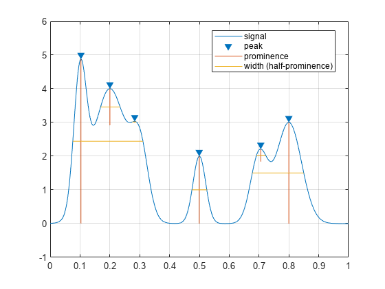
findpeaks(y,x,MinPeakProminence=4,Annotate="extents")

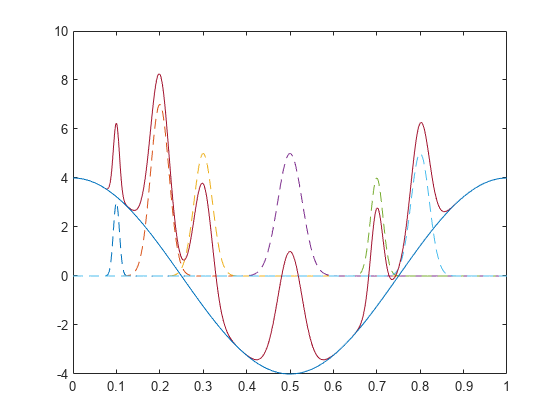
Display the location, prominence, and peak width at half prominence of all the peaks. The second and fourth peaks are the ones with prominence greater than or equal to 4.

[~,locs,widths,proms] = findpeaks(y,x)

locs = 1×6

    0.1001    0.1982    0.2983    0.4995    0.7017    0.8018

widths = 1×6

    0.0154    0.0431    0.0377    0.0625    0.0274    0.0409

proms = 1×6

    2.6816    5.5773    3.1448    4.4171    2.9191    3.6363

Find Peaks with Minimum Separation

Extract peaks from sunspot average count data and estimate the average sunspot cycle.

Load the file sunspot.dat, which contains the average number of sunspots observed every year from 1700 to 1987. Plot the number of sunspots by year and overlay the maxima. Zoom into the time period between 1855 and 1920.

load sunspot.dat

year = sunspot(:,1);
avSpots = sunspot(:,2);

findpeaks(avSpots,year)
xlabel("Year")
xlim([1855 1920])

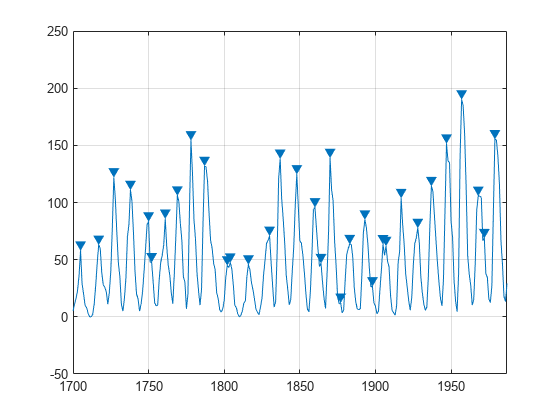
Sunspots are a cyclic phenomenon. Their number is known to peak roughly every 11 years.

Estimate the cycle duration by finding the average separation between peaks. Start by ignoring peaks that are not maxima. Restrict the acceptable peak-to-peak separations to periods greater than 6 years.

findpeaks(avSpots,year,MinPeakDistance=6)
xlabel("Year")
xlim([1855 1920])

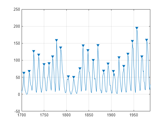
Create a datetime array using the yearly data. Assume the sunspots were counted every year on March 20th, close to the vernal equinox. Find the peak sunspot years. Use the years function to specify the minimum peak separation as a duration.

ty = datetime(year,3,20);
[pk,lk] = findpeaks(avSpots,ty,MinPeakDistance=years(6));
plot(ty,avSpots,lk,pk,"o")
xlabel("Year")

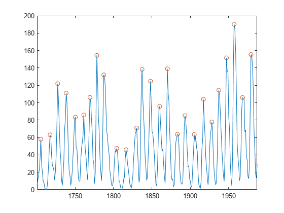
Compute the average sunspot cycle. The estimated average sunspot cycle closely agrees with the known 11-year period.

dttmCycle = years(mean(diff(lk)))

dttmCycle = 
10.9600

Constrain Peak Features

You can find peaks that meet certain feature criteria, among them, minimum or maximum peak distance or height, prominence, and threshold of peak difference with its neighbors. Use findpeaks to constrain single or multiple peak features.

Constrain Peaks by Feature from Audio Signal

Load an audio signal sampled at 7418 Hz. Select 200 samples.

load mtlb
select = mtlb(1001:1200);

Find and highlight all the peaks from the audio signal. Then, find and highlight the peaks that are separated by at least 5 ms. To apply the minimum separation constraint, findpeaks chooses the tallest peak in the signal and eliminates all peaks within 5 ms of it. The function then repeats the procedure for the tallest remaining peak and iterates until it runs out of peaks to consider.

figure
tiledlayout("vertical")
nexttile
findpeaks(select,Fs)
legend("No Constraints",Location="southwest")
nexttile
lgn = @(txt) legend(txt,FontName="FixedWidth",Location="southwest");
findpeaks(select,Fs,MinPeakDistance=0.005)
lgn("MinPeakDistance")

Find and plot the peaks that individually meet each of these constraints:

• Find the peaks with an amplitude of at least 1 V.

• Find the peaks that are at least 1 V higher than their neighboring samples.

• Find the peaks that drop at least 1 V on either side before the signal attains a higher value.

figure
tiledlayout("vertical")
nexttile
findpeaks(select,Fs,MinPeakHeight=1)
lgn("MinPeakHeight")
nexttile
findpeaks(select,Fs,Threshold=1)
lgn("Threshold")
nexttile
findpeaks(select,Fs,MinPeakProminence=1)
lgn("MinPeakProminence")

Constrain Multiple Peak Features from Chirp Signal

Find and highlight all peaks of a 1000-sample chirp signal whose widths are between 2.5 and 4 ms.

N = 1000;
x = sin(2*pi*(1:N)/N + (10*(1:N)/N).^2);
figure
findpeaks(x,Fs,Annotate="extents", ...
    MinPeakWidth=2.5e-3,MaxPeakWidth=4e-3)
title("Peaks with Multiple Constraints")

Peaks and Valleys of Saturated Signal

Sensors can return clipped readings if the data are larger than a given saturation point. You can choose to disregard these extrema as meaningless or incorporate them to your analysis.

Generate a signal that consists of a product of trigonometric functions of frequencies 5 Hz and 3 Hz embedded in white Gaussian noise of variance 0.1². Sample the signal for one second at a rate of 100 Hz. Reset the random number generator for reproducible results.

rng("default")

Fs = 100;
t = 0:1/Fs:1;

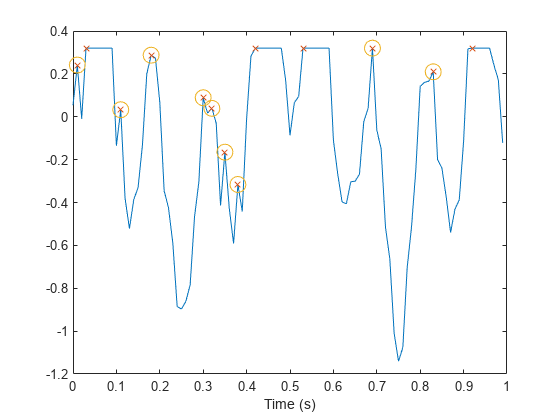
s = sin(2*pi*5*t).*sin(2*pi*3*t) + randn(size(t))/10;

Synthesize a saturated measurement by truncating every reading where the absolute value is greater than the specified bound of 0.32. Then, normalize the signal and make it range between 0.1 and 1. Convert the normalized magnitude to decibels and plot the result.

bnd = 0.32;
s(s>bnd) = bnd;
s(s<-bnd) = -bnd;
sNorm = 0.1+0.9*(s-min(s))/(max(s)-min(s));
sig = mag2db(sNorm);

plot(t,sig)
xlabel("Time (s)")
ylabel("Magnitude (dB)")
ylim([-25 5])

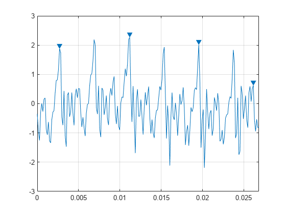
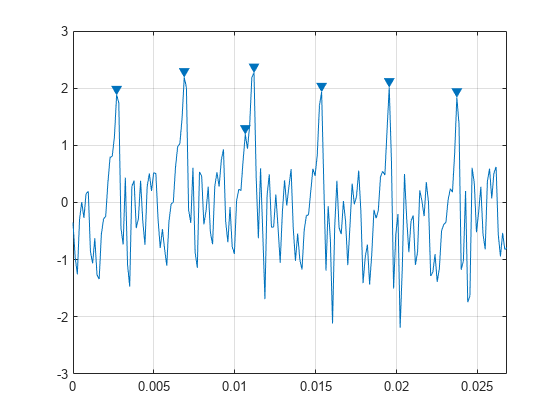
Locate the peaks and valleys of the signal. findpeaks identifies only the rising edge of each flat peak.

[pk,lcp] = findpeaks(sig,t);  % Peaks
[vl,lcv] = findpeaks(-sig,t); % Valleys

hold on
plot(lcp,pk,"x",lcv,-vl,"*")

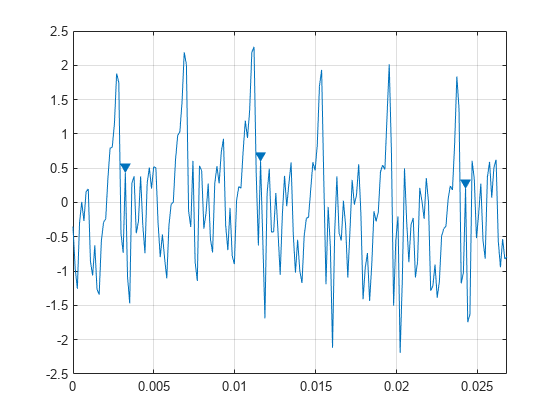
Use the Threshold name-value argument to exclude the flat peaks and valleys. Require a minimum magnitude difference of 0.1 dB between a peak or valley and its neighbors.

[pkt,lctp] = findpeaks(sig,t,Threshold=0.1);
[vlt,lctv] = findpeaks(-sig,t,Threshold=0.1);
plot(lctp,pkt,"o",LineWidth=1.2)
plot(lctv,-vlt,"d",LineWidth=1.2)

Determine Peak Widths

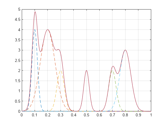
Create a signal that consists of a sum of Gaussian curves. Specify the location, height, and width of each curve.

x = linspace(0,1,1000);

Pos = [1 2 3 5 7 8]'/10;
Hgt = [7 6 3 2 2 3]';
Wdt = [3 8 4 3 4 6]'/100;

y = sum(Hgt.*(exp(-((x-Pos)./Wdt).^2)),1);

Measure the widths of the peaks using half prominence and half height as reference.

tiledlayout("flow")
nexttile
findpeaks(y,x,Annotate="extents")
title("Half-Prominence Peak Widths")
nexttile
findpeaks(y,x,Annotate="extents",WidthReference="halfheight")
title("Half-Height Peak Widths")

Select the tallest peaks separated by at least 0.5 units in the x-axis. Measure the widths of the peaks using half prominence and half height as reference.

figure
tiledlayout("flow")
nexttile
findpeaks(y,x,MinPeakDistance=0.5,Annotate="extents")
title("Half-Prominence Peak Widths")
nexttile
findpeaks(y,x,MinPeakDistance=0.5,Annotate="extents", ...
    WidthReference="halfheight")
title("Half-Height Peak Widths")

Only the first and last peaks satisfy the minimum separation condition, so the widths displayed in the plot correspond to these two peaks. The extent of each peak remains unchanged, so the peak width preserves its value regardless of the conditions specified and whether the peak is selected or not.

Nonlinear Least Squares Peak Refinement

Obtain a refined peak location estimate for the main two peaks in a signal using the nonlinear least squares method with a sinc function kernel.

Generate Signal

Radar pulse compression of a linear FM waveform produces a sinc-shaped spectrum, where the frequency locations of the peaks are proportional to the distance between the radar and the detected object. You can first estimate the peak locations and amplitudes with findpeaks and then enhance your estimates with refinepeaks. This example finds the peak amplitudes and locations of a synthetic noiseless pulse compression signal and uses refinepeaks to improve the estimates.

Generate a signal composed of two sinc-shaped waveforms with peaks of 1 and 1.5 at 4.76 kHz and 35.8 kHz, respectively. Set the frequency spacing to 2.5 Hz.

aTg = [1 1.5];
fTg = 1e3*[4.76 35.8];
freqkHzFull = (0:0.0025:50)';
waveFull = abs(sinc([1 0.5].*(freqkHzFull-fTg/1e3)))*aTg';

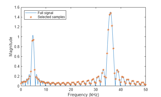
Downsample the signal by a factor of 200 so the frequency spacing between samples is 0.5 kHz. This example refines the amplitude and location estimates of the downsampled signal peaks and compares the improved estimates to the values in the original signals.

freq = downsample(freqkHzFull,200);
wave = downsample(waveFull,200);

plot(freqkHzFull,waveFull,freq,wave,"*")
legend(["Full signal" "Selected samples"],Location="northwest")
xlabel("Frequency (kHz)")
ylabel("Magnitude")

Refine Peaks Using Nonlinear Least Squares

Use findpeaks to make initial estimates of the amplitudes, locations, and half-height widths of the two highest peaks of the signal.

[PV,PL,PW] = findpeaks(wave,NPeaks=2, ...
    SortStr="descend",WidthReference="halfheight");
table(PV,freq(PL), RowNames="Peak estimate "+(1:numel(PV)), ...
    VariableNames=["Amplitude" "Frequency (kHz)"])

ans=2×2 table
                       Amplitude    Frequency (kHz)
                       _________    _______________

    Peak estimate 1     1.4824            36       
    Peak estimate 2     0.9374             5       

Use refinepeaks to enhance the peak estimation using the nonlinear least squares (NLS) method. Specify the frequency points of the signal and the peak widths. The peak values are significantly closer to the expected values of 1.5 and 1, while the frequency locations approximate well to 35.8 kHz and 4.76 kHz, respectively.

LW = max(PW,2);
[Ypk,Xpk] = refinepeaks(wave,PL,freq,Method="NLS",LobeWidth=LW);
table(Ypk,Xpk, RowNames="Refined peak "+(1:numel(Ypk)), ...
    VariableNames=["Amplitude" "Frequency (kHz)"])

ans=2×2 table
                      Amplitude    Frequency (kHz)
                      _________    _______________

    Refined peak 1     1.5063            35.8     
    Refined peak 2     1.0163          4.7628     

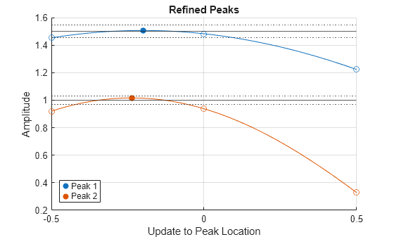
Plot the amplitudes of the refined peaks on the y-axis and the updated peak locations compared with the initial peak estimates on the x-axis. The two initially estimated peaks and their two surrounding samples are each separated by 0.5 kHz. The refined peaks, indicated by filled circles, show the actual peak locations compared to the initially estimated peak locations as well as the corrected amplitudes.

refinepeaks(wave,PL,freq,Method="NLS",LobeWidth=LW)
yline(aTg) % Theoretical peak amplitudes
errorBounds = aTg.*(1+0.03*[-1;1]);
yline(errorBounds(:),":") % ±3% error bounds
legend("Peak "+[1 2])

Input Arguments

y — Input data

vector

Input data, specified as a vector. y must be real-valued and must have at least three elements.

Data Types: double | single

x — Locations

vector | datetime array

Locations, specified as a vector or a datetime array. x must increase monotonically and have the same length as y. If you omit x, then the function uses the indices of y as locations.

Data Types: double | single | datetime

Fs — Sample rate

positive scalar

Sample rate, specified as a positive scalar. The sample rate is the number of samples per unit time. If the unit of time is seconds, the sample rate has units of hertz.

Data Types: double | single

Name-Value Arguments

Specify optional pairs of arguments as Name1=Value1,...,NameN=ValueN, where Name is the argument name and Value is the corresponding value. Name-value arguments must appear after other arguments, but the order of the pairs does not matter.

Example: findpeaks(y,x,SortStr="descend",NPeaks=3) finds the three tallest peaks of the signal y.

NPeaks — Maximum number of peaks

positive integer scalar

Maximum number of peaks to return, specified as a positive integer scalar.

• If you do not specify this argument, findpeaks returns all the peaks identified from the input data y.

• If you specify this argument as NPeaks=np, findpeaks returns up to np peaks from the input data y. If you also specify SortStr, findpeaks returns the peaks as follows:

  • If SortStr="none", findpeaks returns the first np peaks from the input data.

  • If SortStr="ascend", findpeaks returns np peaks in ascending order, starting with the shortest peak from the input data.

  • If SortStr="descend", findpeaks returns np peaks in descending order, starting with the tallest peak from the input data.

Data Types: double | single

SortStr — Peak sorting

"none" (default) | "ascend" | "descend"

Peak sorting, specified as one of these values:

• "none" returns the peaks in the order in which they occur in the input data.

• "ascend" returns the peaks in ascending or increasing order, from the smallest to the largest value.

• "descend" returns the peaks in descending order, from the largest to the smallest value.

MinPeakHeight — Minimum peak height

-Inf (default) | real-valued scalar

Minimum peak height, specified as a real-valued scalar. Use MinPeakHeight to have findpeaks return only those peaks that are higher than the value specified in this argument. Specifying a minimum peak height can reduce processing time.

Data Types: double | single

MinPeakProminence — Minimum peak prominence

0 (default) | nonnegative scalar

Minimum peak prominence, specified as a nonnegative scalar. Use MinPeakProminence to have findpeaks return only those peaks that have a relative importance of at least the value specified in this argument. For more information, see Prominence.

Data Types: double | single

Threshold — Minimum height difference

0 (default) | nonnegative scalar

Minimum height difference between a peak and its neighbors, specified as a nonnegative scalar. Use Threshold to have findpeaks return only those peaks that exceed their immediate neighboring values by at least the value specified in this argument.

Data Types: double | single

MinPeakDistance — Minimum peak separation

0 (default) | positive scalar

Minimum peak separation, specified as a positive scalar. When you specify a value MinPeakDistance=d, the findpeaks function chooses the tallest peak in the signal and ignores all peaks within d samples or units of time around the tallest peak found. The function then repeats the procedure for the tallest remaining peak and iterates until it runs out of peaks to consider.

• If you specify a location vector, x, then MinPeakDistance must be expressed in terms of x. If x is a datetime array, then specify MinPeakDistance as a duration scalar or as a numeric scalar expressed in days.

• If you specify a sample rate, Fs, then MinPeakDistance must be expressed in units of time.

• If you specify neither x nor Fs, then MinPeakDistance must be expressed in units of samples.

Use this argument to have findpeaks ignore small peaks that occur in the neighborhood of a larger peak.

Data Types: double | single | duration

WidthReference — Reference height for width measurements

"halfprom" (default) | "halfheight"

Reference height for width measurements, specified as either "halfprom" or "halfheight".

The findpeaks function estimates the width of a peak as the distance between the points where the descending signal intercepts a horizontal reference line. The function selects the height of the line using the criterion specified in this argument:

• "halfprom" positions the reference line beneath the peak at a vertical distance equal to half the peak prominence. See Prominence for more information.

• "halfheight" positions the reference line at one-half the peak height. The function truncates the line if any of its intercept points lie beyond the borders of the peaks that it determines by using the values of the MinPeakHeight, MinPeakProminence, and Threshold arguments. The border between peaks is defined by the horizontal position of the lowest valley between them. The function discards peaks with height less than zero when you select this value.

The function computes the locations of the intercept points by linear interpolation.

MinPeakWidth — Minimum peak width

0 (default) | positive scalar

Minimum peak width, specified as a positive scalar. Specify MinPeakWidth=minPW to select only those peaks that have widths of at least minPW samples or units of time.

• If you specify a location vector, x, then MinPeakWidth must be expressed in terms of x. If x is a datetime array, then specify MinPeakWidth as a duration scalar or as a numeric scalar expressed in days.

• If you specify a sample rate, Fs, then MinPeakWidth must be expressed in units of time.

• If you specify neither x nor Fs, then MinPeakWidth must be expressed in units of samples.

Data Types: double | single | duration

MaxPeakWidth — Maximum peak width

Inf (default) | positive scalar

Maximum peak width, specified as a positive scalar. Use this argument Specify MaxPeakWidth=maxPW to select only those peaks that have widths of at most maxPW samples or units of time.

• If you specify a location vector, x, then MaxPeakWidth must be expressed in terms of x. If x is a datetime array, then specify MaxPeakWidth as a duration scalar or as a numeric scalar expressed in days.

• If you specify a sample rate, Fs, then MaxPeakWidth must be expressed in units of time.

• If you specify neither x nor Fs, then MaxPeakWidth must be expressed in units of samples.

Data Types: double | single | duration

Annotate — Plot style

"peaks" (default) | "extents"

Plot style, specified as one of these values:

• "peaks" plots the signal and annotates the location and value of every peak.

• "extents" plots the signal and annotates the location, value, width, and prominence of every peak.

The function ignores this argument if you call findpeaks with output arguments.

Output Arguments

pks — Local maxima

vector

Local maxima, returned as a vector of signal values. If there are no local maxima, then pks is empty.

locs — Peak locations

vector

Peak locations, returned as a vector.

• If you specify a location vector, x, then locs contains the values of x at the peak indices.

• If you specify a sample rate, Fs, then locs is a numeric vector of time instants with a time difference of 1/Fs between consecutive samples.

• If you specify neither x nor Fs, then locs is a vector of integer indices.

w — Peak widths

vector

Peak widths, returned as a vector of real-valued numbers. The width of each peak is computed as the distance between the points to the left and right of the peak where the signal intercepts a reference line whose height is specified by WidthReference. The points themselves are found by linear interpolation.

• If you specify a location vector, x, then the widths are expressed in terms of x.

• If you specify a sample rate, Fs, then the widths are expressed in units of time.

• If you specify neither x nor Fs, then the widths are expressed in units of samples.

p — Peak prominences

vector

Peak prominences, returned as a vector of real-valued numbers. The prominence of a peak is the minimum vertical distance that the signal must descend on either side of the peak before either climbing back to a level higher than the peak or reaching an endpoint. See Prominence for more information.

More About

Prominence

The prominence of a peak measures how much the peak stands out due to its intrinsic height and its location relative to other peaks. A low isolated peak can be more prominent than one that is higher but is an otherwise unremarkable member of a tall range.

To measure the prominence of a peak:

1. Place a marker on the peak.

2. Extend a horizontal line from the peak to the left and right until the line does one of the following:

   • Crosses the signal because there is a higher peak

   • Reaches the left or right end of the signal

3. Find the minimum of the signal in each of the two intervals defined in Step 2. This point is either a valley or one of the signal endpoints.

4. The higher of the two interval minima specifies the reference level. The height of the peak above this level is its prominence.

findpeaks makes no assumption about the behavior of the signal beyond its endpoints, whatever their height. As a result, Steps 2 and 4 disregard signal behavior beyond endpoints, which often affects the value of the reference level. Consider for example the peaks of this signal:

Peak Number	Left Interval Lies Between Peak and	Right Interval Lies Between Peak and	Lowest Point on the Left Interval	Lowest Point on the Right Interval	Reference Level (Highest Minimum)
1	Left end	Crossing due to peak 2	Left endpoint	a	a
2	Left end	Right end	Left endpoint	h	Left endpoint
3	Crossing due to peak 2	Crossing due to peak 4	b	c	c
4	Crossing due to peak 2	Crossing due to peak 6	b	d	b
5	Crossing due to peak 4	Crossing due to peak 6	d	e	e
6	Crossing due to peak 2	Right end	d	h	d
7	Crossing due to peak 6	Crossing due to peak 8	f	g	g
8	Crossing due to peak 6	Right end	f	h	f
9	Crossing due to peak 8	Crossing due to right endpoint	h	i	i

Tips

You can initially estimate signal peaks with findpeaks, and then enhance their amplitudes and locations with refinepeaks.

Assume you have a signal with amplitudes y and locations x. This code snippet shows how you can estimate and refine peaks from y and x.

[yPeaks,xPeaksIdx] = findpeaks(y);
[yRPeaks,xRPeaks] = refinepeaks(y,xPeaksIdx,x)

Extended Capabilities

C/C++ Code Generation

Generate C and C++ code using MATLAB® Coder™.

Usage notes and limitations:

• The findpeaks function does not support datetime inputs for code generation.

GPU Code Generation

Generate CUDA® code for NVIDIA® GPUs using GPU Coder™.

Usage notes and limitations:

• The findpeaks function does not support datetime inputs for code generation.

GPU Arrays

Accelerate code by running on a graphics processing unit (GPU) using Parallel Computing Toolbox™.

This function fully supports GPU arrays. For more information, see Run MATLAB Functions on a GPU (Parallel Computing Toolbox).

Version History

Introduced in R2007b

R2024b: findpeaks supports GPU Code Generation

The findpeaks function supports code generation for graphical processing units (GPUs). You must have MATLAB^® Coder™ and GPU Coder™ to generate CUDA^® code.