pwelch

Welch’s power spectral density estimate

Syntax

pxx = pwelch(x)

[pxx,f] = pwelch(x,win,nOverlap,freqSpec)

[pxx,f] = pwelch(x,win,nOverlap,freqSpec,Fs)

[___] = pwelch(___,freqRange,spectrumType,trace)

[___,pxxc] = pwelch(___,ConfidenceLevel=p)

[___] = pwelch(___,Parent=h)

pwelch(___)

Description

pxx = pwelch(x) returns the power spectral density (PSD) estimate of the signal x using Welch's overlapped segment averaging estimator. The function treats the columns of x as independent channels.

[pxx,f] = pwelch(x,win,nOverlap,freqSpec) returns Welch's PSD estimate of the signal x and the frequencies f (rad/sample), where the pwelch function:

• Uses win to divide the signal into segments and windows them.

• Uses the overlap length specified in nOverlap to overlap samples between adjoining segments.

• Computes the discrete Fourier transform (DFT) of each windowed segment over the number of DFT points or at the frequencies specified in freqSpec.

To use default values for any of these input arguments, specify them as empty, [].

[pxx,f] = pwelch(x,win,nOverlap,freqSpec,Fs) specifies the sample rate Fs and returns the cyclical frequencies f in Hz.

[___] = pwelch(___,freqRange,spectrumType,trace) also specifies the frequency range, spectrum type, and trace mode for any of the previous syntaxes. You can specify any combination of these input arguments.

[___,pxxc] = pwelch(___,ConfidenceLevel=p) returns the p × 100% confidence intervals for the PSD estimate in pxxc.

[___] = pwelch(___,Parent=h) plots the Welch PSD estimate or power spectrum in the target parent container h.

pwelch(___) with no output arguments plots the Welch PSD estimate or power spectrum in the current figure window.

Examples

Welch Estimate Using Default Inputs

Obtain the Welch PSD estimate of an input signal consisting of a discrete-time sinusoid with an angular frequency of $$\pi /4$$ rad/sample with additive $$N(0,1)$$ white noise.

Create a sine wave with an angular frequency of $$\pi /4$$ rad/sample with additive $$N(0,1)$$ white noise. Reset the random number generator for reproducible results. The signal has a length $$N_x=320$$ samples.

rng("default")

n = 0:319;
x = cos(pi/4*n) + randn(size(n));

Obtain the Welch PSD estimate using the default Hamming window and DFT length. The default segment length is 71 samples and the DFT length is the 256 points yielding a frequency resolution of $$2\pi /256$$ rad/sample. Because the signal is real-valued, the periodogram is one-sided and there are 256/2+1 points. Plot the Welch PSD estimate.

pxx = pwelch(x);

pwelch(x)

Repeat the computation.

• Divide the signal into sections of length $$nsc=\lfloor N_x/4.5\rfloor$$. This action is equivalent to dividing the signal into the longest possible segments to obtain as close to but not exceed 8 segments with 50% overlap.

• Window the sections using a Hamming window.

• Specify 50% overlap between contiguous sections

• To compute the FFT, use $$\max (256,2^p)$$ points, where $$p=\lceil {\log }_{2}nsc\rceil$$.

Verify that the two approaches give identical results.

Nx = length(x);
nsc = floor(Nx/4.5);
nov = floor(nsc/2);
nff = max(256,2^nextpow2(nsc));

pxxt = pwelch(x,hamming(nsc),nov,nff);

maxerr = max(abs(abs(pxxt(:)) - abs(pxx(:))))

maxerr = 
0

Divide the signal into 8 sections of equal length, with 50% overlap between sections. Specify the same FFT length as in the preceding step. Compute the Welch PSD estimate and verify that it gives the same result as the previous two procedures.

ns = 8;
ov = 0.5;
lsc = floor(Nx/(ns-(ns-1)*ov));

pxxt8 = pwelch(x,lsc,floor(ov*lsc),nff);

maxerr8 = max(abs(abs(pxxt8(:)) - abs(pxx(:))))

maxerr8 = 
0

Welch Estimate Using Specified Segment Length

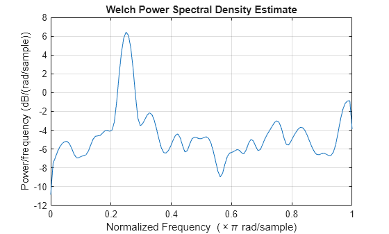
Obtain the Welch PSD estimate of an input signal consisting of a discrete-time sinusoid with an angular frequency of $$\pi /3$$ rad/sample with additive $$N(0,1)$$ white noise.

Create a sine wave with an angular frequency of $$\pi /3$$ rad/sample with additive $$N(0,1)$$ white noise. Reset the random number generator for reproducible results. The signal has 512 samples.

rng("default")

n = 0:511;
x = cos(pi/3*n) + randn(size(n));

Obtain the Welch PSD estimate dividing the signal into segments 132 samples in length. The signal segments are multiplied by a Hamming window 132 samples in length. The number of overlapped samples is not specified, so it is set to 132/2 = 66. The DFT length is 256 points, yielding a frequency resolution of $$2\pi /256$$ rad/sample. Because the signal is real-valued, the PSD estimate is one-sided and there are 256/2+1 = 129 points. Plot the PSD as a function of normalized frequency.

segmentLength = 132;
[pxx,w] = pwelch(x,segmentLength);

plot(w/pi,pow2db(pxx))
xlabel("Normalized Frequency (\times \pi rad/sample)")
title("Welch Power Spectral Density Estimate")

Welch Estimate Specifying Segment Overlap

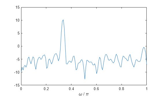
Obtain the Welch PSD estimate of an input signal consisting of a discrete-time sinusoid with an angular frequency of $$\pi /4$$ rad/sample with additive $$N(0,1)$$ white noise.

Create a sine wave with an angular frequency of $$\pi /4$$ rad/sample with additive $$N(0,1)$$ white noise. Reset the random number generator for reproducible results. The signal is 320 samples in length.

rng("default")

n = 0:319;
x = cos(pi/4*n) + randn(size(n));

Obtain the Welch PSD estimate dividing the signal into segments 100 samples in length. The signal segments are multiplied by a Hamming window 100 samples in length. The number of overlapped samples is 25. The DFT length is 256 points yielding a frequency resolution of $$2\pi /256$$ rad/sample. Because the signal is real-valued, the PSD estimate is one-sided and there are 256/2+1 points.

segmentLength = 100;
noverlap = 25;
pxx = pwelch(x,segmentLength,noverlap);

plot(pow2db(pxx))
xlabel("Frequency Samples")
title("Welch Power Spectral Density Estimate")

Welch Estimate Using Specified DFT Length

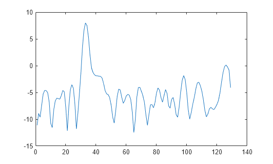
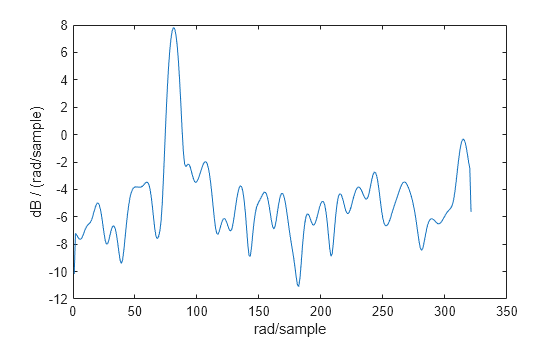
Obtain the Welch PSD estimate of an input signal consisting of a discrete-time sinusoid with an angular frequency of $$\pi /4$$ rad/sample with additive $$N(0,1)$$ white noise.

Create a sine wave with an angular frequency of $$\pi /4$$ rad/sample with additive $$N(0,1)$$ white noise. Reset the random number generator for reproducible results. The signal is 320 samples in length.

rng("default")

n = 0:319;
x = cos(pi/4*n) + randn(size(n));

Obtain the Welch PSD estimate dividing the signal into segments 100 samples in length. Use the default overlap of 50%. Specify the DFT length to be 640 points so that the frequency of $$\pi /4$$ rad/sample corresponds to a DFT bin (bin 81). Because the signal is real-valued, the PSD estimate is one-sided and there are 640/2+1 points.

segmentLength = 100;
nfft = 640;
pxx = pwelch(x,segmentLength,[],nfft);

plot(pow2db(pxx))
xlabel("Frequency Points")
title("Welch Power Spectral Density Estimate")

Welch PSD Estimate of Signal with Frequency in Hertz

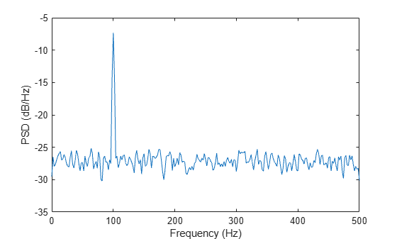
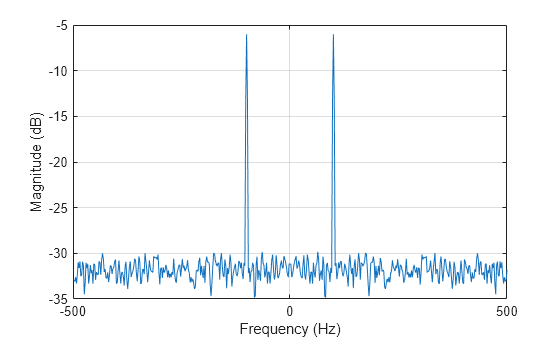
Create a signal consisting of a 100 Hz sinusoid in additive N(0,1) white noise. Reset the random number generator for reproducible results. The sample rate is 1 kHz and the signal is 5 seconds in duration.

rng("default")

Fs = 1000;
t = 0:1/Fs:5-1/Fs;
x = cos(2*pi*100*t) + randn(size(t));

Obtain Welch's overlapped segment averaging PSD estimate of the preceding signal. Use a segment length of 500 samples with 300 overlapped samples. Use 500 DFT points so that 100 Hz falls directly on a DFT bin. Input the sample rate to output a vector of frequencies in Hz. Plot the result.

[pxx,f] = pwelch(x,500,300,500,Fs);

plot(f,pow2db(pxx))

xlabel("Frequency (Hz)")
ylabel("PSD (dB/Hz)")

Maximum-Hold and Minimum-Hold Spectra

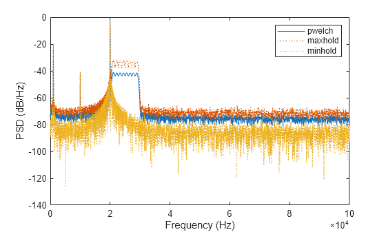
Create a signal consisting of three noisy sinusoids and a chirp, sampled at 200 kHz for 0.1 second. The frequencies of the sinusoids are 1 kHz, 10 kHz, and 20 kHz. The sinusoids have different amplitudes and noise levels. The noiseless chirp has a frequency that starts at 20 kHz and increases linearly to 30 kHz during the sampling.

rng("default")
Fs = 200e3; 
Fc = [1 10 20]'*1e3; 
Ns = 0.1*Fs;

t = (0:Ns-1)/Fs;
x = [1 1/10 10]*sin(2*pi*Fc*t) + [1/200 1/2000 1/20]*randn(3,Ns);
x = x + chirp(t,20e3,t(end),30e3);

Compute the Welch PSD estimate and the maximum-hold and minimum-hold spectra of the signal. Plot the results.

[pxx,f] = pwelch(x,[],[],[],Fs);
pmax = pwelch(x,[],[],[],Fs,"maxhold");
pmin = pwelch(x,[],[],[],Fs,"minhold");

plot(f,pow2db(pxx))
hold on
plot(f,pow2db([pmax pmin]),":")
hold off
xlabel("Frequency (Hz)")
ylabel("PSD (dB/Hz)")
legend(["pwelch" "maxhold" "minhold"])

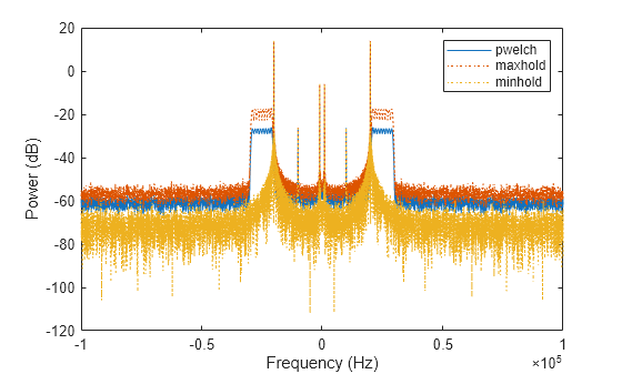
Repeat the procedure, this time computing centered power spectrum estimates.

[pxx,f] = pwelch(x,[],[],[],Fs,"centered","power");
pmax = pwelch(x,[],[],[],Fs,"maxhold","centered","power");
pmin = pwelch(x,[],[],[],Fs,"minhold","centered","power");

plot(f,pow2db(pxx))
hold on
plot(f,pow2db([pmax pmin]),":")
hold off
xlabel("Frequency (Hz)")
ylabel("Power (dB)")
legend(["pwelch" "maxhold" "minhold"])

Upper and Lower 95%-Confidence Bounds

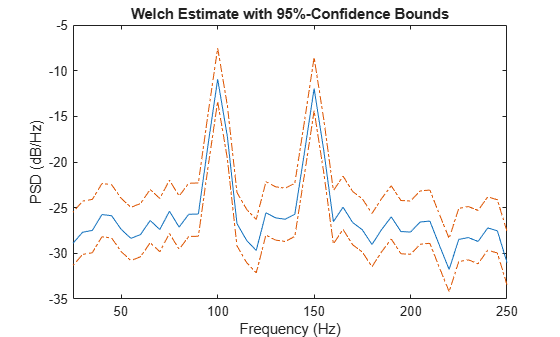
This example illustrates the use of confidence bounds with Welch's overlapped segment averaging (WOSA) PSD estimate. While not a necessary condition for statistical significance, frequencies in Welch's estimate where the lower confidence bound exceeds the upper confidence bound for surrounding PSD estimates clearly indicate significant oscillations in the time series.

Create a signal consisting of the superposition of 100 Hz and 150 Hz sine waves in additive white N(0,1) noise. The amplitude of the two sine waves is 1. The sample rate is 1 kHz. Reset the random number generator for reproducible results.

rng("default")
Fs = 1000;
t = 0:1/Fs:1-1/Fs;
x = cos(2*pi*100*t) + sin(2*pi*150*t) + randn(size(t));

Obtain the WOSA estimate with 95%-confidence bounds. Set the segment length equal to 200 and overlap the segments by 50% (100 samples).

L = 200;
win = hamming(L);
nOverlap = 100;
[pxx,f,pxxc] = pwelch(x,win,nOverlap,200,Fs,ConfidenceLevel=0.95);

Plot the WOSA PSD estimate along with the confidence interval and zoom in on the frequency region of interest near 100 and 150 Hz. The lower confidence bound in the immediate vicinity of 100 and 150 Hz is significantly above the upper confidence bound outside the vicinity of 100 and 150 Hz.

plot(f,pow2db(pxx))
hold on
plot(f,pow2db(pxxc),"-.",Color=[0.866 0.329 0])
hold off

xlim([25 250])
xlabel("Frequency (Hz)")
ylabel("PSD (dB/Hz)")
title("Welch Estimate with 95%-Confidence Bounds")

DC-Centered Power Spectrum

Create a signal consisting of a 100 Hz sinusoid in additive $$N(0,1/4)$$ white noise. Reset the random number generator for reproducible results. The sample rate is 1 kHz and the signal is 5 seconds in duration.

rng("default")

Fs = 1000;
t = 0:1/Fs:5-1/Fs;

noisevar = 1/4;
x = cos(2*pi*100*t) + sqrt(noisevar)*randn(size(t));

Obtain the DC-centered power spectrum using Welch's method. Use a segment length of 500 samples with 300 overlapped samples and a DFT length of 500 points.

[pxx,f] = pwelch(x,500,300,500,Fs,"centered","power");

Plot the result. The power at -100 and 100 Hz is close to the expected power of 1/4 for a real-valued sine wave with an amplitude of 1. The deviation from 1/4 is due to the effect of the additive noise.

plot(f,pow2db(pxx))
xlabel("Frequency (Hz)")
ylabel("Magnitude (dB)")
grid

Welch PSD Estimate of a Multichannel Signal

Generate 1024 samples of a multichannel signal consisting of three sinusoids in additive $$N(0,1)$$ white Gaussian noise. The sinusoids' frequencies are $$\pi /2$$, $$\pi /3$$, and $$\pi /4$$ rad/sample. Estimate the PSD of the signal using Welch's method and plot it.

N = 1024;
n = 0:N-1;

w = pi./[2;3;4];

rng("default")
x = cos(w*n)' + randn(length(n),3);

pwelch(x)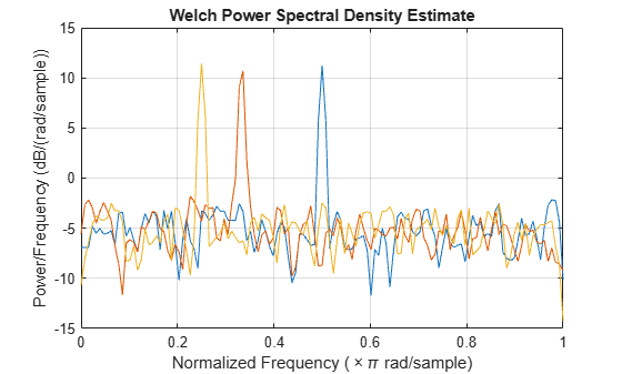

Plot Welch PSD in Target Axes and Panel Container

Since R2026a

Plot the Welch power spectral density (PSD) estimate and Welch power spectrum for four signals in the specified target axes and panel containers.

Create four oscillating signals with a sample rate of 10 kHz for three seconds.

Fs = 10e3;
t = 0:1/Fs:3;
x1 = sinc(Fs/2.5*(t-mean(t)));
x2 = sum(cos(2*pi*600*[1 3 5 7]'.*t),1) + randn(size(t))/1e4;
x3 = exp(1j*pi*sin(4*t)*Fs/10);
x4 = chirp(t,Fs/10,t(end),Fs/2.5,"quadratic");

Plot Welch PSD Estimate and Power Spectrum in Target Axes

Create two axes in the southwestern and northeastern corners of a new figure window.

fig = figure;
ax1 = axes(fig,Position=[0.09 0.1 0.52 0.45]);
ax2 = axes(fig,Position=[0.55 0.7 0.42 0.25]);

Plot the Welch PSD estimate and Welch power spectrum of the signals x1 and x2 in the southwestern and northeastern axes of the figure, respectively. Use a 256-sample Kaiser window, an overlap length of 220 samples, and 512 DFT points.

g = kaiser(256,5);
ol = 220;
nfft = 512;

pwelch(x1,g,ol,nfft,Fs,Parent=ax1)
pwelch(x2,g,ol,nfft,Fs,"power",Parent=ax2)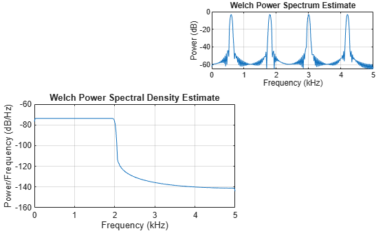

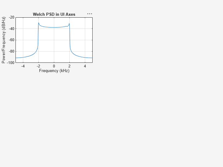
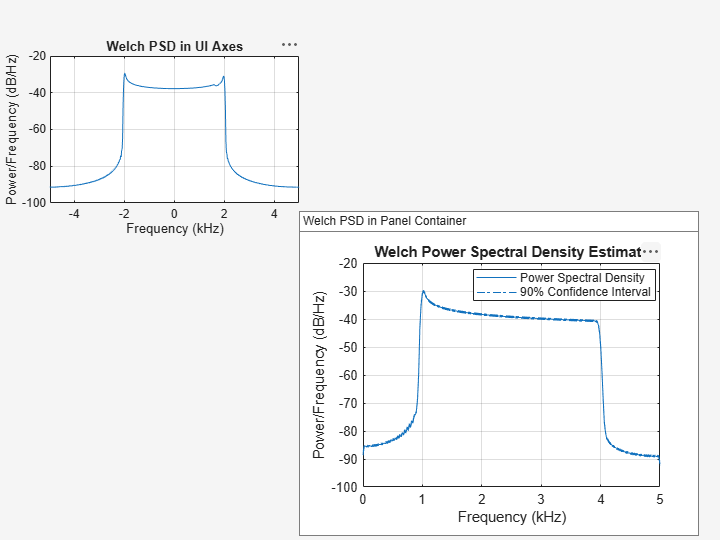
Plot Welch PSD Estimate in Target UI Axes

Create an axes in the northwestern corner of a new UI figure window.

uif = uifigure(Position=[100 100 720 540]);
ax3 = uiaxes(uif,Position=[5 305 300 200]);

Plot the Welch PSD estimate of the signal x3 on the figure axes. Display the frequencies centered at 0 kHz.

pwelch(x3,g,ol,nfft,Fs,"centered",Parent=ax3)
title(ax3,"Welch PSD in UI Axes")

Plot Welch PSD Estimate in Target Panel Container

Add a panel container in the southeastern corner of the UI figure window.

p = uipanel(uif,Position=[300 5 400 325], ...
    Title="Welch PSD in Panel Container", ...
    BackgroundColor="white");

Plot the Welch PSD estimate of the signal x4 on the panel container. Set the confidence level to 90%.

pwelch(x4,g,ol,nfft,Fs,ConfidenceLevel=0.9,Parent=p)

Input Arguments

x — Input signal

vector | matrix

Input signal, specified as a vector or as a matrix. If you specify x as a matrix, then pwelch treats its columns as independent channels.

Example: cos(pi/4*(0:159))+randn(1,160) is a single-channel row-vector signal.

Example: cos(pi./[4;2]*(0:159))'+randn(160,2) is a two-channel signal.

Data Types: single | double
Complex Number Support: Yes

win — Window

[] (default) | positive integer | vector

Window, specified as empty ([]), a positive integer, or a vector.

The pwelch function divides the input signal x into segments and uses a window to compute the element-by-element product of the segment samples and the window values. The window values depend on the how you specify this argument.

• Empty ([]) — pwelch uses a Hamming window of length such that x is divided into eight segments with nOverlap overlapping samples.

• Positive integer — pwelch divides x into segments of length win and uses a Hamming window of that length.

• Vector — pwelch divides x into segments of the same length as the vector win and uses the window specified in win.

If the length of x cannot be divided exactly into an integer number of segments with nOverlap overlapping samples, then pwelch truncates x accordingly.

For a list of available windows, see Windows.

Note

The default Hamming window has a 42.5 dB sidelobe attenuation, which may mask spectral content below this value (relative to the peak spectral content). Choosing different windows enables you to make tradeoffs between resolution (for example, using a rectangular window) and sidelobe attenuation (for example, using a Hann window). See Window Designer for more details.

Example: hann(N+1) and (1-cos(2*pi*(0:N)'/N))/2 both specify a Hann window of length N + 1.

Data Types: single | double

nOverlap — Number of overlapped samples

[] (default) | nonnegative integer

Number of overlapped samples, specified as empty ([]) or a nonnegative integer.

• Empty ([]) — pwelch uses a number that produces 50% overlap between segments.

  If the segment length is unspecified, the function sets nOverlap to ⌊N_x / 4.5⌋, where N_x is the length of the input signal and the ⌊ ⌋ symbols denote the floor function. This action is equivalent to dividing the signal into the longest possible segments to obtain as close to but not exceed eight segments with 50% overlap.

• Nonnegative integer — pwelch overlaps adjoining segments using the number of samples specified in this argument.

  • If win is scalar, then nOverlap must be smaller than win.

  • If win is a vector, then nOverlap must be smaller than the length of win.

freqSpec — Frequency specification

[] (default) | positive integer | vector

Frequency specification, specified as one of these values:

• Empty, [] — pwelch calculates the spectral estimates using a number of DFT points equal to the greater of 256 or the next power of two that is equal or larger than the window length.

• Positive integer — pwelch calculates the spectral estimates using the number of DFT points specified in this argument.

  • If freqSpec is greater than the segment length, then pwelch pads the segment data with zeros.

  • If freqSpec is less than the segment length, then pwelch partitions the segment modulo freqSpec and sums the resulting segment frames.

• Vector of at least two elements — pwelch calculates the spectral estimates at the frequencies specified in freqSpec.

  • If you specify the sample rate, Fs, pwelch assumes freqSpec as cyclical frequencies in the same units as of Fs.

  • If you do not specify Fs, pwelch assumes freqSpec as normalized frequencies in rad/sample.

Example: freqSpec = 512 specifies 512 DFT points.

Example: freqSpec = pi./[8 4 2] specifies a vector of three normalized frequencies.

Data Types: single | double

Fs — Sample rate

positive scalar

Sample rate, specified as a positive scalar. The sample rate is the number of samples per unit time. If the unit of time is seconds, then the sample rate is in Hz.

• If you specify Fs as empty [], then pwelch assumes that the input signal x has a sample rate of 1 Hz.

• If you do not specify Fs, then pwelch assumes that the input signal x has a sample rate of 2π rad/sample.

freqRange — Frequency range for PSD estimate or power spectrum

"onesided" | "twosided" | "centered"

Frequency range of the PSD estimate or power spectrum, specified as "onesided", "twosided", or "centered".

The pwelch function returns pxx with a number of rows and frequency interval that depends on the value specified in freqRange, whether the number of DFT points freqSpec is even or odd, and whether Fs is specified or not.

freqRange	freqSpec	Number of Rows in pxx	Frequency Interval for pxx
			Fs unspecified	Fs specified
"onesided" (default if x is real-valued)	Even	freqSpec/2 + 1	[0,π] rad/sample	[0,Fs/2] cycles/unit time
	Odd	(freqSpec + 1)/2	[0,π) rad/sample	[0,Fs/2) cycles/unit time
"twosided" (default if x is complex-valued)	Even or odd	freqSpec	[0,2π) rad/sample	[0,Fs) cycles/unit time
"centered"	Even	freqSpec	(–π,π] rad/sample	(–Fs/2,Fs/2] cycles/unit time
	Odd		(–π,π) rad/sample	(–Fs/2,Fs/2) cycles/unit time

Note

• This argument is not supported if you specify freqSpec as a vector of cyclical or normalized frequencies.

• If you specify the "onesided" value, pwelch multiplies the power by 2 at all frequencies except 0 and the Nyquist frequency to conserve the total power.

• The "onesided" value is not supported if x is complex-valued.

Data Types: char | string

spectrumType — Power spectrum scaling

"psd" (default) | "power"

Power spectrum scaling, specified as one of these values:

• "psd" — pwelch returns the power spectral density.

• "power" — pwelch scales each estimate of the PSD by the equivalent noise bandwidth of the window and returns an estimate of the power at each frequency.

This table shows the scaling relation between the PSD estimate and power spectrum estimate, either of both returned in pxx, given an input signal x, window vector win, overlap length nOverlap, frequency specification freqSpec, and sample rate Fs.

Sample Rate	Scaling Relation
Fs specified	psd = pwelch(x,win,nOverlap,freqSpec,Fs,"psd"); pow = pwelch(x,win,nOverlap,freqSpec,Fs,"power"); Then, pow is equivalent to psd*enbw(win,Fs). win is a window vector.
Fs unspecified	psd = pwelch(x,win,nOverlap,freqSpec,"psd"); pow = pwelch(x,win,nOverlap,freqSpec,"power"); Then, pow is equivalent to psd*enbw(win,2*pi).

trace — Trace mode

"mean" (default) | "maxhold" | "minhold"

Trace mode, specified as one of these values:

• "mean" — pwelch returns Welch's spectrum estimate of each input channel by averaging the power spectrum estimates across all the segments at each frequency bin.

• "maxhold" — pwelch returns the maximum-hold spectrum of each input channel by selecting the maximum power spectrum value across segments at each frequency bin.

• "minhold" — pwelch returns the minimum-hold spectrum of each input channel by selecting the minimum power spectrum value across segments at each frequency bin.

p — Confidence interval for PSD estimate

0.95 (default) | scalar in the range (0,1)

Coverage probability for the PSD estimate, specified as a scalar in the range (0,1).

If you specify ConfidenceLevel=p and pxxc, the function outputs pxxc with the lower and upper bounds of the p × 100% interval estimate for the true PSD.

h — Target parent container

[] (default) | Axes object | UIAxes object | Panel object

Since R2026a

Target parent container, specified as an Axes object, a UIAxes object, or a Panel object.

If you specify Parent=h, the pwelch function plots the Welch PSD estimate or power spectrum on the specified target parent container, whether you call the function with or without output arguments.

For more information about target containers and the parent-child relationship in MATLAB^® graphics, see Graphics Object Hierarchy. For more information about using Parent in UIAxes and Panel objects to design apps, see Plot Spectral Representations of Signal in App Designer.

Example: h = axes(figure,Position=[0.1 0.1 0.6 0.5]) defines an axes parent container. When you specify pwelch(x,[],[],[],Parent=h), the function plots the Welch PSD of the input signal x in the parent container h.

Output Arguments

pxx — PSD estimate or power spectrum

vector | matrix

PSD estimate or power spectrum, returned as a real-valued, nonnegative column vector or matrix.

• Each column of pxx is the PSD estimate or the or power spectrum of the corresponding column of x and depending on how you specify spectrumType.

• The units of the PSD estimate are in squared-magnitude units of the input signal per unit frequency. For example, if the input data x is in volts, you specify the sample rate Fs in hertz, and you assume a resistance of 1 Ω, then the PSD estimate is in watts per hertz.

• The units of the power spectrum are in squared-magnitude units of the input signal. For example, if the input data x is in volts and you assume a resistance of 1 Ω, then the PSD estimate is in watts.

f — Frequencies associated with PSD estimate

vector

Frequencies associated with the PSD estimate, returned as a real-valued column vector.

• If you specify Fs, then f contains cyclical frequencies in Hz.

• If you do not specify Fs, then f contains normalized frequencies in rad/sample.

pxxc — Confidence bounds

matrix

Confidence bounds, returned as a real-valued matrix.

• pxxc has the same number of rows as in pxx.

• pxxc has twice as many columns as pxx.

  • Odd-numbered columns contain the lower bounds of the confidence intervals.

  • Even-numbered columns contain the upper bounds of the confidence intervals.

  Thus, pxxc(m,2*n-1) is the lower confidence bound and pxxc(m,2*n) is the upper confidence bound corresponding to the estimate pxx(m,n).

• The coverage probability of the confidence intervals is determined by the value of the p input.

Data Types: single | double

More About

Welch’s Overlapped Segment Averaging Spectral Estimation

The periodogram is not a consistent estimator of the true power spectral density of a wide-sense stationary process. Welch’s technique to reduce the variance of the periodogram breaks the input signal into overlapping segments.

Welch’s method computes a modified periodogram for each segment and then averages these estimates to produce the estimate of the power spectral density. Because the process is wide-sense stationary and Welch’s method uses PSD estimates of different segments of the input signal, the modified periodograms represent approximately uncorrelated estimates of the true PSD and averaging reduces the variability.

The segments are typically multiplied by a window function, such as a Hamming window, so that Welch’s method amounts to averaging modified periodograms. Because the segments usually overlap, data values at the beginning and end of the segment tapered by the window in one segment, occur away from the ends of adjacent segments. This guards against the loss of information caused by windowing.

References

[1] Hayes, Monson H. Statistical Digital Signal Processing and Modeling. New York: John Wiley & Sons, 1996.

[2] Stoica, Petre, and Randolph Moses. Spectral Analysis of Signals. Upper Saddle River, NJ: Prentice Hall, 2005.

Extended Capabilities

Tall Arrays

Calculate with arrays that have more rows than fit in memory.

The pwelch function supports tall arrays with the following usage notes and limitations:

• The input x must not be a tall row vector

• The win argument must always be specified.

For more information, see Tall Arrays.

C/C++ Code Generation
Generate C and C++ code using MATLAB® Coder™.

GPU Code Generation
Generate CUDA® code for NVIDIA® GPUs using GPU Coder™.

Thread-Based Environment

Run code in the background using MATLAB® backgroundPool or accelerate code with Parallel Computing Toolbox™ ThreadPool.

The pwelch function supports thread-based environments with these usage notes and limitations:

• The syntax with no output arguments is not supported.

For more information, see Run MATLAB Functions in Thread-Based Environment.

GPU Arrays

Accelerate code by running on a graphics processing unit (GPU) using Parallel Computing Toolbox™.

This function fully supports GPU arrays. For more information, see Run MATLAB Functions on a GPU (Parallel Computing Toolbox).

Version History

Introduced before R2006a

R2026a: Visualize function outputs in specified parent targets

The pwelch function supports plotting output in a parent axes or panel container specified using the Parent input argument.

R2024b: pwelch supports GPU Code Generation

The pwelch function supports code generation for graphical processing units (GPUs). You must have MATLAB Coder™ and GPU Coder™ to generate CUDA^® code.

R2024a: Code generation support for single-precision variable-size window inputs

The pwelch function supports single-precision variable-size window inputs for code generation.

R2023b: Use single-precision data

The pwelch function supports single-precision inputs.

R2023a: Visualize function outputs using Create Plot Live Editor task

You can now use the Create Plot Live Editor task to visualize the output of pwelch interactively. You can select different chart types and set optional parameters. The task also automatically generates code that becomes part of your live script.