Quadrotor Trajectory Tracking Using Iterative Learning Control

R2026b

Since R2025a

This example demonstrates quadrotor trajectory tracking control using the Iterative Learning Control (ILC) block in Simulink® Control Design™. ILC is used in the outer-loop position control for quadrotor trajectory tracking. The quadrotor is commanded to track a circular trajectory, the vehicle is also subjected to external aerodynamic disturbance caused by wind bias. This example uses ILC over repeated iterations and the controller learns to minimize error and improve tracking of a given reference signal.

Quadrotor Model

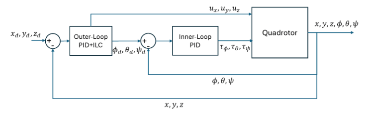
This example demonstrates the quadrotor trajectory control using PID augmented by ILC controller. Quadrotor use two-loop cascaded control. The outer-loop control the position of the vehicle in x-y-z in the inertial frame. The inner-loop controls the attitude of the vehicle yaw-pitch-roll also in inertial frame. You use Iterative learning control in the outer loop along with the PID for position control. The inner-loop use a stand-alone PID controller.

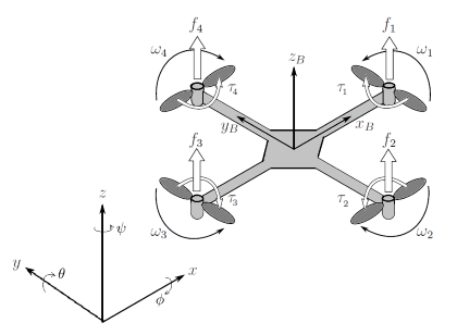
For a 6-DOF quadrotor model, consider the following:

• $u,v,w$ are the vehicle velocity in the body frame.

• $p,q,r$ are the angular velocity of the vehicle in body frame.

• $\text{Roll}-\varphi ,\text{Pitch}-\theta ,\text{Yaw}-\psi$are defined in vehicle-2, vehicle-1 and vehicle frame respectively.

• $x,y,z$ is the vehicle translation motion in inertial frame.

This example uses simplified quadrotor dynamics that with the following assumptions:

• Assume the $\text{Roll}-\varphi$ and $\text{Pitch}-\theta$angles are small and hence body rates are approximately equal to inertial rates,

$$\left[\begin{array}{c}\underset{}{\overset{\dot{}}{\varphi }}\\ \underset{}{\overset{\dot{}}{\theta }}\\ \underset{}{\overset{\dot{}}{\psi }}\end{array}\right]=\left[\begin{array}{c}\underset{}{\overset{\dot{}}{p}}\\ \underset{}{\overset{\dot{}}{q}}\\ \underset{}{\overset{\dot{}}{r}}\end{array}\right]$$

• Assume affect of Coriolis components are negligible, $\text{qr},\text{pr},\text{pq}\approx 0$.

• In this example you will control position and attitude. Heading angle $\text{Yaw}-\psi$is assumed to be held zero.

With these simplifying assumptions, the quadrotor model can be written as [1],

• Outer-Loop quadrotor dynamics for position in inertial frame:

$$\begin{array}{l}\underset{}{\overset{¨}{x}}=-\cos \left(\varphi \right)\sin \left(\theta \right)\frac{F}{m}\\ \underset{}{\overset{¨}{y}}=\sin \left(\varphi \right)\frac{F}{m}\\ \underset{}{\overset{¨}{z}}=g-\cos \left(\varphi \right)\cos \left(\theta \right)\frac{F}{m}\end{array}$$

• Inner-Loop quadrotor dynamics of attitude angles in inertial frame:

$$\begin{array}{l}\underset{}{\overset{¨}{\varphi }}=\frac{1}{J_x}\tau {}_{\varphi }\\ \underset{}{\overset{¨}{\theta }}=\frac{1}{J_y}\tau {}_{\theta }\\ \underset{}{\overset{¨}{\psi }}=\frac{1}{J_z}\tau {}_{\psi }\end{array}$$

Here, $F=f_1+f_2+f_3+f_4$ is the total propeller forces,$\tau {}_{\varphi },\tau {}_{\theta },\tau {}_{\psi }$are the torques applied to the quadrotor, $m$ is vehicle mass, and $g=9.81$ is the gravitational constant.

Two-Loop Controller for Quadrotor Trajectory Tracking

The following image shows the two-loop cascaded control architecture for the quadrotor. The outer loop generates the translation forces to control the position of the vehicle. The inner loop tracks the reference attitude angles and generates body torques.

Simplifying the outer-loop translation equation of motion, you can define following control terms.

$$\begin{array}{l}{u}_x=-\cos \left(\varphi \right)\sin \left(\theta \right)\frac{F}{m}\\ u_y=\sin \left(\varphi \right)\frac{F}{m}\\ u_z=g-\cos \left(\varphi \right)\cos \left(\theta \right)\frac{F}{m}\end{array}$$

Here, $u_x$, $u_y$, and $u_z$ are the outputs of the outer-loop PID controller for quadrotor position. Using these three outer-loop control signals, you can solve for the commanded roll ${\varphi }_d$, pitch ${\theta }_d$, and yaw ${\psi }_d$ as reference signals for inner-loop control.

$\begin{array}{l}{\varphi }_d={\tan }^{-1}\left(\frac{u_y\cos \left(\theta \right)}{g-u_z}\right)\\ {\theta }_d={\tan }^{-1}\left(\frac{u_x}{u_z-g}\right)\\ {\psi }_d=0\end{array}$.

The inner loop implements a PID controller to track the commanded reference attitude angles ${\varphi }_d$, ${\theta }_d$, and ${\psi }_d$.

Quadrotor Trajectory Tracking

The goal of this example is to have the quadrotor track a circular trajectory. The quadrotor starts at initial position $\left[x_0,y_0,z_0\right]=\left[\begin{array}{ccc}3& 0& 1\end{array}\right]$ in the inertial frame and executes a circle of radius $R=3m$. The time for quadrotor to complete one circle trajectory is $\text{Tspan}=15\sec$.

% Set the Circular trajectory radius
R = 3;

% Quadrotor initial condition in inertial frame
IC = [3 0 -1]; % In North-East-Down co-ordinate frame

Outer Loop Position Control PID

The outer-loop control for the quadrotor tracks the reference trajectory in the x-y-z frame. The following image shows the three-axis independent controller for the quadrotor. The controller gains can be tuned one at a time using the successive loop closure method.

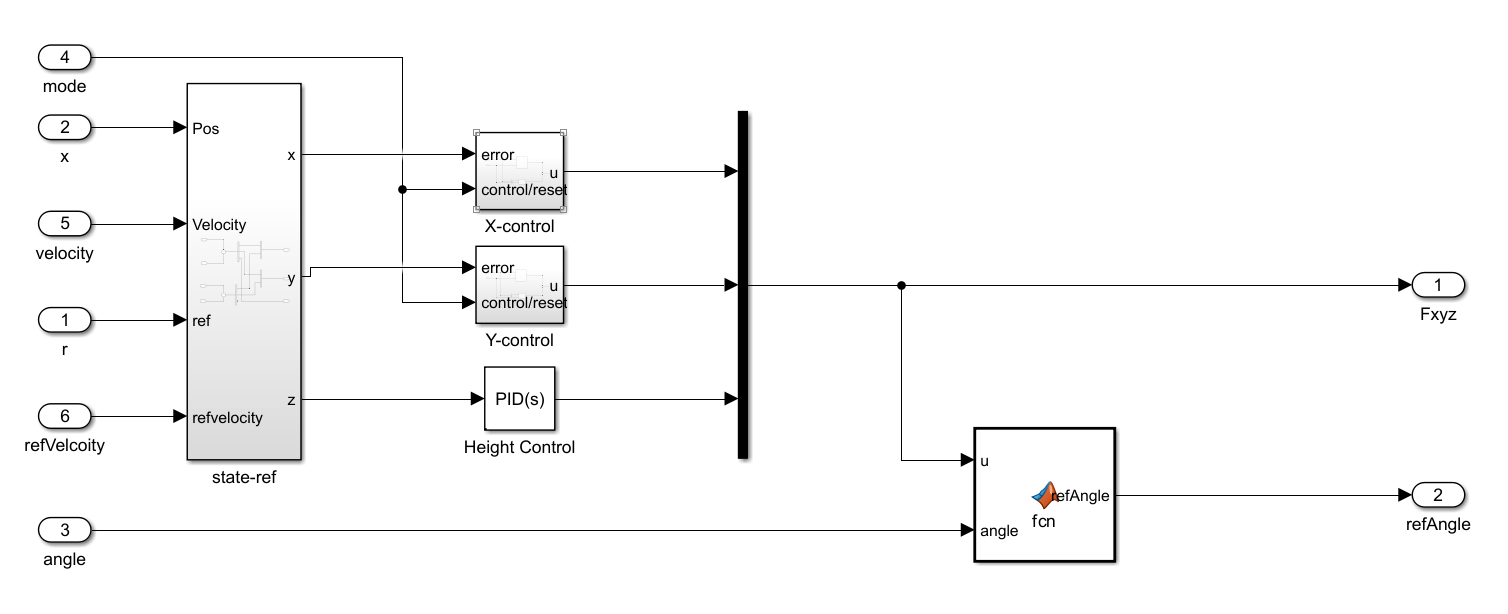
The individual control loops in $X$, $Y$, and $Z$, have baseline PID controllers designed to track the trajectory, such that $x\to x_d$, $y\to y_d$, and $z\to z_d$.

$$u_{\xi }=k_{p_{\xi }}\left({\xi }_d-\xi \right)+k_{d_{\xi }}\left(\underset{}{\overset{\dot{}}{{\xi }_d}}-\underset{}{\overset{\dot{}}{\xi }}\right)+k_{I_{\xi }}\int \left({\xi }_d-\xi \right)\text{dt}$$

Here, state $\xi =\left[\begin{array}{ccc}x& y& z\end{array}\right]\text{and}{\xi }_d=\left[\begin{array}{ccc}{x}_d& y_d& z_d\end{array}\right]$.

Specify tuned controller gains for the $X$ and $Y$ control loops.

% X-axis PID gains
Kp_x = 1;
Kd_x = 0.97;
Ki_x = 0.01;

% Y-Axis PID Gains
Kp_y = 0.1;
Kd_y = 2.5;
Ki_y = 0.01;

Iterative Learning Control Overview

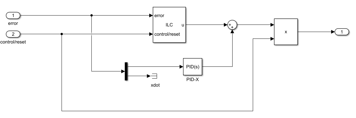
The $X$ and $Y$ outer-loop position control are augmented with ILC control. Where as height (Z) is a standalone PID controller, designed to maintain the height at $Z=1m$. The quadrotor repeats the circular trajectory for $K$ iterations. The ILC controller goal is to iteratively improve tracking performance. A brief description of ILC control is as follows, for more details see Iterative Learning Control.

Iterative learning control (ILC) is an improvement in run-to-run control. It uses frequent measurements in the form of the error trajectory from the previous batch to update the control signal for the subsequent batch run. The focus of ILC has been on improving the performance of systems that execute a single, repeated operation, starting at the same initial operating condition. This focus includes many practical industrial systems in manufacturing, robotics, and chemical processing, where mass production on an assembly line entails repetition.

• Suitable for repetitive task + repetitive disturbances.

• Use knowledge from previous iteration to improve next iteration.

A general model based ILC control update is as follows [2],

$$u_{k+1}\left(t\right)=Q\left(q\right)\left[u_k\left(t\right)+L\left(q\right)e_k\left(t+1\right)\right]$$

Where L is learning function based on the system model G. In this example you use inverse model ILC, which use learning function $L=G^{-1}$. where G is the input-output relation for LTI system, in the lifted form as follows $y_k={\text{Gu}}_k+d$.

ILC Modes

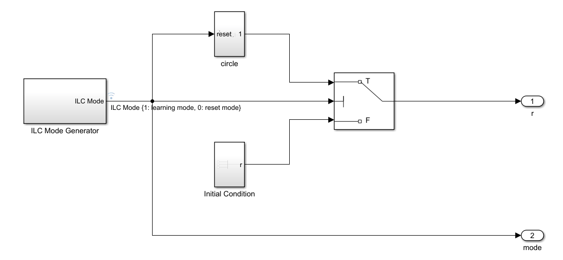
At runtime, ILC switches between two modes: control and reset. In the control mode, ILC outputs $u_k\left(t\right)$at the desired time points and measures the error between the desired reference $r\left(t\right)$ and output $y_k\left(t\right)$. At the end of the control mode, ILC calculates the new control sequence $u_{k+1}\left(t\right)$ to use in the next iteration. In the reset mode, ILC output is 0. The reset mode must be long enough such that the return to home controller in this mode brings the plant back to its initial condition.

ILC Design

To design an ILC controller, configure these parameters:

• Sample time and iteration duration — These parameters determine how many control actions ILC provides in control mode. If the sample time is too large, ILC might not provide sufficient compensation. If the sample time is too small, ILC might take too many resources. In particular, it might create a large memory footprint when using model-based ILC.

• Model information — This example use model based ILC. A nominal closed loop model information is necessary to design the ILC controller.

• ILC gains — The controller gains determine how well ILC learns between iterations. If the ILC gains are too big, it might make the closed-loop system unstable (robustness). If the ILC gains are too small, it might lead to slower convergence (performance).

• Low-pass filter time constant — The optional low-pass filter removes control chatter, which might otherwise be amplified during learning. By default, this filter it is not enabled in the ILC block.

Define the parameters for the ILC block.

% Sample Time
Ts = 0.05;

% Single iteration duration
Tspan = 15;

In this example, you use a model-based ILC approach. The nominal discrete model for the $X$ and $Y$ axes has the following state-space matrices.

A = [1 0.05;-0.02 0.97];
B = [0;0.05];
C = eye(2);

Specify the ILC gains for the $X$ and $Y$ axes.

gamma_x = 0.3;
gamma_y = 0.08;

ILC implements a low-pass filter to remove high-gain control oscillations. This filter adds a tradeoff between rate of convergence and robustness. Specify the time constant for the filter.

% Filter Coeff
Filter_coeff = 2;

Inner-Loop Attitude Control PID

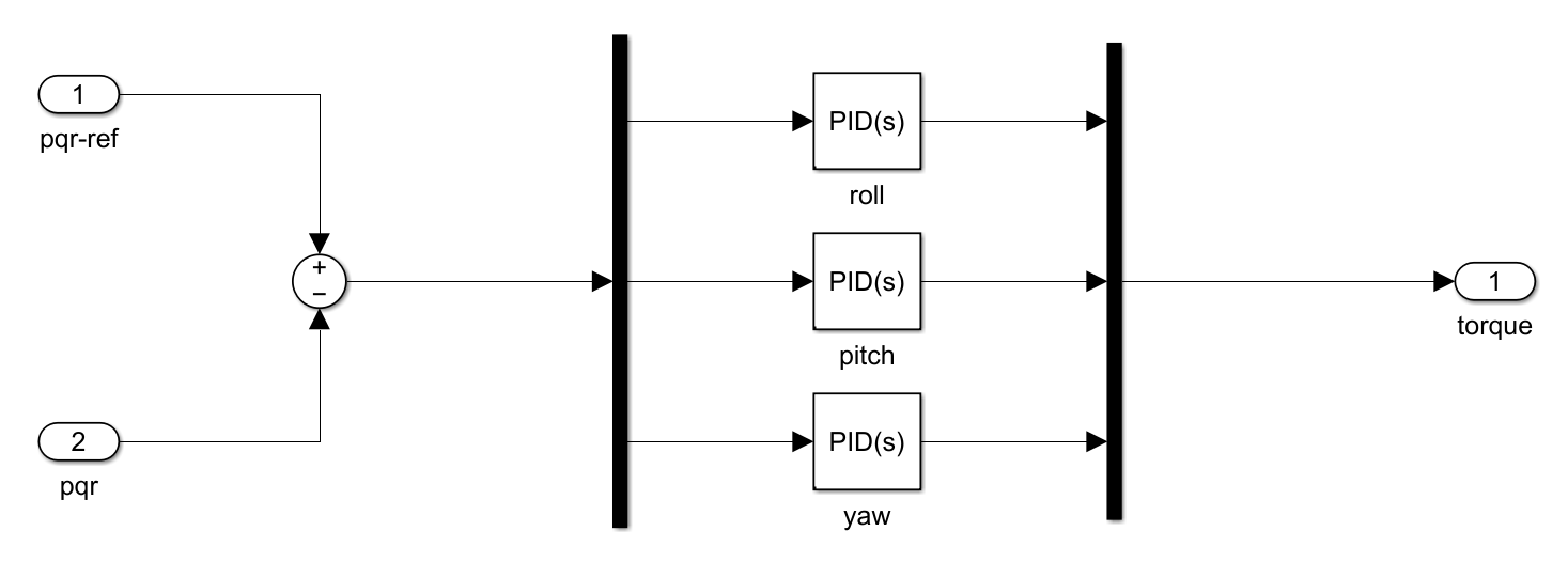
The inner-loop controllers for the quadrotor track the reference attitudes. The roll, pitch, and yaw control loops each have baseline PID controllers designed to track their respective reference attitudes such that $\varphi \to {\varphi }_d$, $\theta \to {\theta }_d$, and $\psi \to {\psi }_d$.

$$\tau {}_{\xi }=k_{p_{\xi }}\left({\xi }_d-\xi \right)+k_{d_{\xi }}\left(\underset{}{\overset{\dot{}}{{\xi }_d}}-\underset{}{\overset{\dot{}}{\xi }}\right)+k_{I_{\xi }}\int \left({\xi }_d-\xi \right)\text{dt}$$

where $\xi =\left[\begin{array}{ccc}\varphi & \theta & \psi \end{array}\right]\text{and}{\xi }_d=\left[\begin{array}{ccc}{\varphi }_d& {\theta }_d& {\psi }_d\end{array}\right]$

you do not augment the baseline PID in the inner loop with ILC. The PID controller gains $k_{p_{\xi }}$, $k_{d_{\xi }}$, and $k_{I_{\xi }}$can be tuned one at a time using successive loop closures. In this example, you use PID autotuning in for the PID Controller block.

Simulate Model and Plot Results

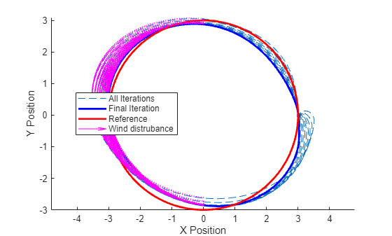
To make the problem more challenging, you add an external wind disturbance to the vehicle. The disturbance is also repetitive in nature and adds drag in $Y$ direction. The wind disturbance in $Y$ direction is modeled as follows,

$$f_{\text{dragY}}=\frac{1}{2}\text{Cd}\rho u_y^2\text{if}x>0,\text{else}{f}_{\text{dragY}}=0$$

where $C_d=0.1$ is coefficient of drag, $\rho =1\frac{\text{kg}}{m^3}$ is density of air and $u_y$ is vehicle velocity in Y direction.

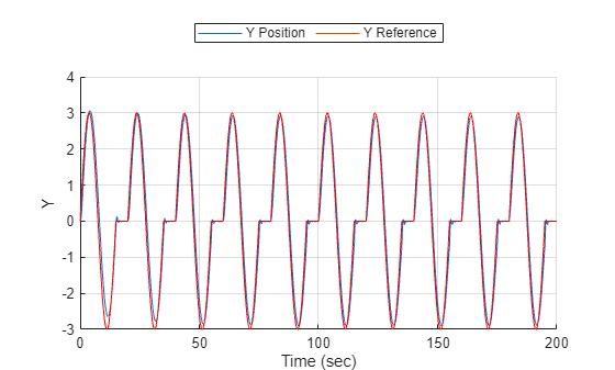
Simulate the model for 10 iterations. In the first iteration, ILC controller outputs 0 in the control mode because it just starts learning. Therefore, the closed-loop control performance displayed in the first iteration comes from the nominal controller, which serves as the baseline for the comparison.

mdl = "quadTrajTrackingILC";
open_system(mdl)
simout = sim(mdl);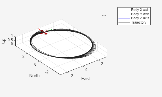

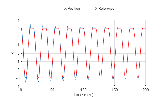
As the iterations progress, the ILC controller improves the reference tacking performance in both the $X$ and $Y$ direction.

Plot the quadrotor tracking performance in the $X$ direction.

figure
hold on
grid on
plot(simout.tout,simout.x.Data)
plot(simout.tout,simout.r.Data(:,1),Color="r")
xlabel("Time (sec)")
ylabel("X")
legend("X Position","X Reference", ...
Location="northoutside",Orientation="horizontal")

Plot the quadrotor tracking performance in the $Y$ direction.

figure
hold on
grid on
plot(simout.tout,simout.y.Data)
plot(simout.tout,simout.r.Data(:,2),Color="r")
xlabel("Time (sec)")
ylabel("Y")
legend("Y Position","Y Reference", ...
Location="northoutside",Orientation="horizontal")

Get the final trajectory index.

final_traj_idx = find(simout.tout >=180);

Plot the quadrotor trajectory in the $XY$ plane

figure
hold on
plot(simout.x.Data(1:final_traj_idx(1)-1), ...
simout.y.Data(1:final_traj_idx(1)-1),"--")
plot(simout.x.Data(final_traj_idx), ...
simout.y.Data(final_traj_idx),LineWidth=2,Color="b")
plot(simout.r.Data(final_traj_idx,1), ...
simout.r.Data(final_traj_idx,2),LineWidth=2,Color="r")
xlabel("X Position")
ylabel("Y Position")

% Plot Wind disturbance vector plot
quiver(simout.x.data(:,1),simout.y.data(:,1), ...
simout.wind.Data(:,1),simout.wind.Data(:,2),Color = "m")
axis equal

legend("All Iterations","Final Iteration", ...
"Reference","Wind distrubance",Location="best")

Plot the control effort in the outer-loop PID+ILC controller.

figure
f = tiledlayout(2,2,TileSpacing="tight");

Plot ILC control effort for the $X$ direction.

nexttile
plot(squeeze(simout.ux_ilc.Data))
xlabel("Time")
ylabel("u")
title("ILC Control X-axis")

Plot PID control effort for the $X$ direction.

nexttile
plot(squeeze(simout.ux_pid.data))
xlabel("Time")
ylabel("u")
title("PID Control X-axis")

Plot ILC control effort for the $Y$ direction.

nexttile
plot(squeeze(simout.uy_ilc.data))
xlabel("Time")
ylabel("u");
title("ILC Control Y-axis")

Plot PID control effort for the $Y$ direction.

nexttile
plot(squeeze(simout.uy_pid.data))
xlabel("Time")
ylabel("u")
title("PID Control Y-axis")

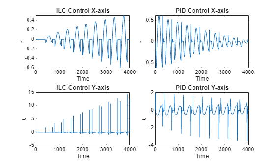
As iterations progress, the ILC controller learns to compensate for the tracking error and the nominal PID control effort is reduced to a minimum.

Reference

[1] Beard, Randal. "Quadrotor dynamics and control rev 0.1." (2008).

[2] Bristow, Douglas A., Marina Tharayil, and Andrew G. Alleyne. “A Survey of Iterative Learning Control.” IEEE Control Systems 26, no. 3 (June 2006): 96–114.