resubMargin

Resubstitution classification margins for multiclass error-correcting output codes (ECOC) model

Syntax

m = resubMargin(Mdl)

m = resubMargin(Mdl,Name,Value)

Description

m = resubMargin(Mdl) returns the resubstitution classification margins (m) for the multiclass error-correcting output codes (ECOC) model Mdl using the training data stored in Mdl.X and the corresponding class labels stored in Mdl.Y.

m is returned as a numeric column vector with the same length as Mdl.Y. The software estimates each entry of m using the trained ECOC model Mdl, the corresponding row of Mdl.X, and the true class label Mdl.Y.

m = resubMargin(Mdl,Name,Value) returns the classification margins with additional options specified by one or more name-value pair arguments. For example, you can specify a decoding scheme, binary learner loss function, and verbosity level.

Examples

Resubstitution Classification Margins of ECOC Model

Calculate the resubstitution classification margins for an ECOC model with SVM binary learners.

Load Fisher's iris data set. Specify the predictor data X and the response data Y.

load fisheriris
X = meas;
Y = species;

Train an ECOC model using SVM binary classifiers. Standardize the predictors using an SVM template, and specify the class order.

t = templateSVM('Standardize',true);
classOrder = unique(Y)

classOrder = 3×1 cell
    {'setosa'    }
    {'versicolor'}
    {'virginica' }

Mdl = fitcecoc(X,Y,'Learners',t,'ClassNames',classOrder);

t is an SVM template object. During training, the software uses default values for empty properties in t. Mdl is a ClassificationECOC model.

Calculate the classification margins for the observations used to train Mdl. Display the distribution of the margins using a box plot.

m = resubMargin(Mdl);

boxplot(m)
title('In-Sample Margins')

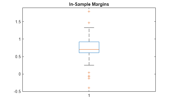
The classification margin of an observation is the positive-class negated loss minus the maximum negative-class negated loss. Choose classifiers that yield relatively large margins.

Select ECOC Model Features by Examining Training-Sample Margins

Perform feature selection by comparing training-sample margins from multiple models. Based solely on this comparison, the model with the greatest margins is the best model.

Load Fisher's iris data set. Define two data sets:

• fullX contains all four predictors.

• partX contains the sepal measurements only.

load fisheriris
X = meas;
fullX = X;
partX = X(:,1:2);
Y = species;

Train an ECOC model using SVM binary learners for each predictor set. Standardize the predictors using an SVM template, specify the class order, and compute posterior probabilities.

t = templateSVM('Standardize',true);
classOrder = unique(Y)

classOrder = 3×1 cell
    {'setosa'    }
    {'versicolor'}
    {'virginica' }

FullMdl = fitcecoc(fullX,Y,'Learners',t,'ClassNames',classOrder,...
    'FitPosterior',true);
PartMdl = fitcecoc(partX,Y,'Learners',t,'ClassNames',classOrder,...
    'FitPosterior',true);

Compute the resubstitution margins for each classifier. For each model, display the distribution of the margins using a boxplot.

fullMargins = resubMargin(FullMdl);
partMargins = resubMargin(PartMdl);

boxplot([fullMargins partMargins],'Labels',{'All Predictors','Two Predictors'})
title('Training-Sample Margins')

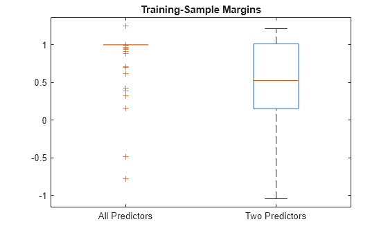
The margin distribution of FullMdl is situated higher and has less variability than the margin distribution of PartMdl. This result suggests that the model trained with all the predictors fits the training data better.

Input Arguments

Mdl — Full, trained multiclass ECOC model

ClassificationECOC model

Full, trained multiclass ECOC model, specified as a ClassificationECOC model trained with fitcecoc.

Name-Value Arguments

Specify optional pairs of arguments as Name1=Value1,...,NameN=ValueN, where Name is the argument name and Value is the corresponding value. Name-value arguments must appear after other arguments, but the order of the pairs does not matter.

Before R2021a, use commas to separate each name and value, and enclose Name in quotes.

Example: resubMargin(Mdl,'Verbose',1) specifies to display diagnostic messages in the Command Window.

BinaryLoss — Binary learner loss function

"hamming" | "linear" | "logit" | "exponential" | "binodeviance" | "hinge" | "quadratic" | function handle

Binary learner loss function, specified as a built-in loss function name or function handle.

• This table describes the built-in functions, where y_j is the class label for a particular binary learner (in the set {–1,1,0}), s_j is the score for observation j, and g(y_j,s_j) is the binary loss formula.

  Value	Description	Score Domain	g(yj,sj)
  "binodeviance"	Binomial deviance	(–∞,∞)	log[1 + exp(–2yjsj)]/[2log(2)]
  "exponential"	Exponential	(–∞,∞)	exp(–yjsj)/2
  "hamming"	Hamming	[0,1] or (–∞,∞)	[1 – sign(yjsj)]/2
  "hinge"	Hinge	(–∞,∞)	max(0,1 – yjsj)/2
  "linear"	Linear	(–∞,∞)	(1 – yjsj)/2
  "logit"	Logistic	(–∞,∞)	log[1 + exp(–yjsj)]/[2log(2)]
  "quadratic"	Quadratic	[0,1]	[1 – yj(2sj – 1)]2/2

  The software normalizes binary losses so that the loss is 0.5 when y_j = 0. Also, the software calculates the mean binary loss for each class [1].

• For a custom binary loss function, for example customFunction, specify its function handle BinaryLoss=@customFunction.

  customFunction has this form:

  bLoss = customFunction(M,s)

  • M is the K-by-B coding matrix stored in Mdl.CodingMatrix.

  • s is the 1-by-B row vector of classification scores.

  • bLoss is the classification loss. This scalar aggregates the binary losses for every learner in a particular class. For example, you can use the mean binary loss to aggregate the loss over the learners for each class.

  • K is the number of classes.

  • B is the number of binary learners.

  For an example of passing a custom binary loss function, see Predict Test-Sample Labels of ECOC Model Using Custom Binary Loss Function.

This table identifies the default BinaryLoss value, which depends on the score ranges returned by the binary learners.

Assumption	Default Value
All binary learners are any of the following: Classification decision trees Discriminant analysis models k-nearest neighbor models Linear or kernel classification models of logistic regression learners Naive Bayes models	"quadratic"
All binary learners are SVMs or linear or kernel classification models of SVM learners.	"hinge"
All binary learners are ensembles trained by AdaboostM1 or GentleBoost.	"exponential"
All binary learners are ensembles trained by LogitBoost.	"binodeviance"
You specify to predict class posterior probabilities by setting FitPosterior=true in fitcecoc.	"quadratic"
Binary learners are heterogeneous and use different loss functions.	"hamming"

To check the default value, use dot notation to display the BinaryLoss property of the trained model at the command line.

Example: BinaryLoss="binodeviance"

Data Types: char | string | function_handle

Decoding — Decoding scheme

"lossweighted" (default) | "lossbased"

Decoding scheme that aggregates the binary losses, specified as "lossweighted" or "lossbased". For more information, see Binary Loss.

Example: Decoding="lossbased"

Data Types: char | string

Options — Estimation options

[] (default) | structure array

Estimation options, specified as a structure array as returned by statset.

To invoke parallel computing you need a Parallel Computing Toolbox™ license.

Example: Options=statset(UseParallel=true)

Data Types: struct

Verbose — Verbosity level

0 (default) | 1

Verbosity level, specified as 0 or 1. Verbose controls the number of diagnostic messages that the software displays in the Command Window.

If Verbose is 0, then the software does not display diagnostic messages. Otherwise, the software displays diagnostic messages.

Example: Verbose=1

Data Types: single | double

More About

Classification Margin

The classification margin is, for each observation, the difference between the negative loss for the true class and the maximal negative loss among the false classes. If the margins are on the same scale, then they serve as a classification confidence measure. Among multiple classifiers, those that yield greater margins are better.

Binary Loss

The binary loss is a function of the class and classification score that determines how well a binary learner classifies an observation into the class. The decoding scheme of an ECOC model specifies how the software aggregates the binary losses and determines the predicted class for each observation.

Assume the following:

• m_kj is element (k,j) of the coding design matrix M—that is, the code corresponding to class k of binary learner j. M is a K-by-B matrix, where K is the number of classes, and B is the number of binary learners.

• s_j is the score of binary learner j for an observation.

• g is the binary loss function.

• $$\widehat{k}$$ is the predicted class for the observation.

The software supports two decoding schemes:

• Loss-based decoding [2] (Decoding is "lossbased") — The predicted class of an observation corresponds to the class that produces the minimum average of the binary losses over all binary learners.

  $$\widehat{k}=\underset{k}{\text{argmin}}\frac{1}{B}{\displaystyle \sum _{j=1}^B\left|m_{kj}\right|g}(m_{kj},s_j).$$

• Loss-weighted decoding [3] (Decoding is "lossweighted") — The predicted class of an observation corresponds to the class that produces the minimum average of the binary losses over the binary learners for the corresponding class.

  $$\widehat{k}=\underset{k}{\text{argmin}}\frac{{\displaystyle \sum _{j=1}^B\left|m_{kj}\right|g}(m_{kj},s_j)}{{\displaystyle \sum }_{j=1}^B\left|m_{kj}\right|}.$$

  The denominator corresponds to the number of binary learners for class k. [1] suggests that loss-weighted decoding improves classification accuracy by keeping loss values for all classes in the same dynamic range.

The predict, resubPredict, and kfoldPredict functions return the negated value of the objective function of argmin as the second output argument (NegLoss) for each observation and class.

This table summarizes the supported binary loss functions, where y_j is a class label for a particular binary learner (in the set {–1,1,0}), s_j is the score for observation j, and g(y_j,s_j) is the binary loss function.

Value	Description	Score Domain	g(yj,sj)
"binodeviance"	Binomial deviance	(–∞,∞)	log[1 + exp(–2yjsj)]/[2log(2)]
"exponential"	Exponential	(–∞,∞)	exp(–yjsj)/2
"hamming"	Hamming	[0,1] or (–∞,∞)	[1 – sign(yjsj)]/2
"hinge"	Hinge	(–∞,∞)	max(0,1 – yjsj)/2
"linear"	Linear	(–∞,∞)	(1 – yjsj)/2
"logit"	Logistic	(–∞,∞)	log[1 + exp(–yjsj)]/[2log(2)]
"quadratic"	Quadratic	[0,1]	[1 – yj(2sj – 1)]2/2

The software normalizes binary losses so that the loss is 0.5 when y_j = 0, and aggregates using the average of the binary learners [1].

Do not confuse the binary loss with the overall classification loss (specified by the LossFun name-value argument of the resubLoss and resubPredict object functions), which measures how well an ECOC classifier performs as a whole.

Tips

• To compare the margins or edges of several ECOC classifiers, use template objects to specify a common score transform function among the classifiers during training.

References

[1] Allwein, E., R. Schapire, and Y. Singer. “Reducing multiclass to binary: A unifying approach for margin classifiers.” Journal of Machine Learning Research. Vol. 1, 2000, pp. 113–141.

[2] Escalera, S., O. Pujol, and P. Radeva. “Separability of ternary codes for sparse designs of error-correcting output codes.” Pattern Recog. Lett. Vol. 30, Issue 3, 2009, pp. 285–297.

[3] Escalera, S., O. Pujol, and P. Radeva. “On the decoding process in ternary error-correcting output codes.” IEEE Transactions on Pattern Analysis and Machine Intelligence. Vol. 32, Issue 7, 2010, pp. 120–134.

Extended Capabilities

Automatic Parallel Support

Accelerate code by automatically running computation in parallel using Parallel Computing Toolbox™.

To run in parallel, specify the Options name-value argument in the call to this function and set the UseParallel field of the options structure to true using statset:

Options=statset(UseParallel=true)

For more information about parallel computing, see Run MATLAB Functions with Automatic Parallel Support (Parallel Computing Toolbox).

GPU Arrays

Accelerate code by running on a graphics processing unit (GPU) using Parallel Computing Toolbox™.

This function fully supports GPU arrays. For more information, see Run MATLAB Functions on a GPU (Parallel Computing Toolbox).

Version History

Introduced in R2014b