Main Content

fitrqlinear

Train quantile linear regression model

Since R2024b

    Description

    Mdl = fitrqlinear(Tbl,ResponseVarName) returns a trained quantile linear regression model Mdl. The function trains the model using the predictors in the table Tbl and the response values in the ResponseVarName table variable.

    By default, the function uses the median (0.5 quantile).

    Mdl = fitrqlinear(Tbl,formula) returns a quantile linear regression model trained using the sample data in the table Tbl. The input argument formula is an explanatory model of the response and a subset of the predictor variables in Tbl used to fit Mdl.

    Mdl = fitrqlinear(Tbl,Y) returns a quantile linear regression model trained using the predictor variables in the table Tbl and the response values in the vector Y.

    Mdl = fitrqlinear(X,Y) returns a quantile linear regression model trained using the predictors in the matrix X and the response values in the vector Y.

    Mdl = fitrqlinear(___,Name=Value) specifies options using one or more name-value arguments in addition to any of the input argument combinations in previous syntaxes. For example, you can specify the quantiles by using the Quantiles name-value argument.

    example

    [Mdl,AggregateOptimizationResults] = fitrqlinear(___) also returns AggregateOptimizationResults, which contains hyperparameter optimization results when you specify the OptimizeHyperparameters and HyperparameterOptimizationOptions name-value arguments. You must also specify the ConstraintType and ConstraintBounds options of HyperparameterOptimizationOptions. You can use this syntax to optimize on the compact model size instead of the cross-validation loss, and to solve a set of multiple optimization problems that have the same options but different constraint bounds. (since R2025a)

    Note

    Hyperparameter optimization is supported only for models with one quantile.

    Examples

    collapse all

    Fit a quantile linear regression model using the 0.25, 0.50, and 0.75 quantiles.

    Load the carbig data set, which contains measurements of cars made in the 1970s and early 1980s. Create a matrix X containing the predictor variables Acceleration, Displacement, Horsepower, and Weight. Store the response variable MPG in the variable Y.

    load carbig
    X = [Acceleration,Displacement,Horsepower,Weight];
    Y = MPG;

    Delete rows of X and Y where either array has missing values.

    R = rmmissing([X Y]);
    X = R(:,1:end-1);
    Y = R(:,end);

    Partition the data into training data (XTrain and YTrain) and test data (XTest and YTest). Reserve approximately 20% of the observations for testing, and use the rest of the observations for training.

    rng(0,"twister") % For reproducibility of the partition
    c = cvpartition(length(Y),"Holdout",0.20);
    
    trainingIdx = training(c);
    XTrain = X(trainingIdx,:);
    YTrain = Y(trainingIdx);
    
    testIdx = test(c);
    XTest = X(testIdx,:);
    YTest = Y(testIdx);

    Train a quantile linear regression model. Specify to use the 0.25, 0.50, and 0.75 quantiles (that is, the lower quartile, median, and upper quartile). To improve the model fit, change the beta tolerance to 1e-6 instead of the default value 1e-4. Use a ridge (L2) regularization term of 1. Adjusting the regularization term can help prevent quantile crossing.

    Mdl = fitrqlinear(XTrain,YTrain,Quantiles=[0.25,0.50,0.75], ...
        BetaTolerance=1e-6,Lambda=1)
    Mdl = 
      RegressionQuantileLinear
                 ResponseName: 'Y'
        CategoricalPredictors: []
            ResponseTransform: 'none'
                         Beta: [4×3 double]
                         Bias: [17.0004 23.0029 29.5243]
                    Quantiles: [0.2500 0.5000 0.7500]
    
    
      Properties, Methods


    Mdl is a RegressionQuantileLinear model object. You can use dot notation to access the properties of Mdl. For example, Mdl.Beta and Mdl.Bias contain the linear coefficient estimates and estimated bias terms, respectively. Each column of Mdl.Beta corresponds to one quantile, as does each element of Mdl.Bias.

    In this example, you can use the linear coefficient estimates and estimated bias terms directly to predict the test set responses for each of the three quantiles in Mdl.Quantiles. In general, you can use the predict object function to make quantile predictions.

    predictedY = XTest*Mdl.Beta + Mdl.Bias
    predictedY = 78×3
    
       12.3963   16.2569   19.5263
        5.8328   10.1568   12.6058
       17.1726   20.6398   24.9748
       23.3790   28.1122   31.3617
       17.0036   22.5314   23.0539
       16.6120   17.0713   20.1062
       10.9274   12.3302   13.2707
       14.9130   14.6659   12.7100
       16.3103   17.7497   20.8477
       19.6229   25.7109   30.5389
       19.5583   24.6621   30.4345
       12.9525   14.4508   16.0004
       14.8525   16.1338   16.4112
       24.1648   31.1758   33.9310
       15.1039   17.8497   19.2013
          ⋮
    
    
    isequal(predictedY,predict(Mdl,XTest))
    ans = logical
       1


    Each column of predictedY corresponds to a separate quantile (0.25, 0.5, or 0.75).

    Visualize the predictions of the quantile linear regression model. First, create a grid of predictor values.

    minX = floor(min(X))
    minX = 1×4
    
               8          68          46        1613
    
    
    maxX = ceil(max(X))
    maxX = 1×4
    
              25         455         230        5140
    
    
    gridX = zeros(100,size(X,2));
    for p = 1:size(X,2)
        gridp = linspace(minX(p),maxX(p))';
        gridX(:,p) = gridp;
    end

    Next, use the trained model Mdl to predict the response values for the grid of predictor values.

    gridY = predict(Mdl,gridX)
    gridY = 100×3
    
       20.8073   25.4104   29.1436
       20.6991   25.2907   29.0251
       20.5909   25.1711   28.9066
       20.4828   25.0514   28.7881
       20.3746   24.9318   28.6696
       20.2664   24.8121   28.5512
       20.1583   24.6924   28.4327
       20.0501   24.5728   28.3142
       19.9419   24.4531   28.1957
       19.8337   24.3335   28.0772
       19.7256   24.2138   27.9587
       19.6174   24.0941   27.8402
       19.5092   23.9745   27.7217
       19.4011   23.8548   27.6032
       19.2929   23.7351   27.4848
          ⋮


    For each observation in gridX, the predict object function returns predictions for the quantiles in Mdl.Quantiles.

    View the gridY predictions for the second predictor (Displacement). Compare the quantile predictions to the true test data values.

    predictorIdx = 2;
    plot(XTest(:,predictorIdx),YTest,".")
    hold on
    plot(gridX(:,predictorIdx),gridY(:,1))
    plot(gridX(:,predictorIdx),gridY(:,2))
    plot(gridX(:,predictorIdx),gridY(:,3))
    hold off
    xlabel("Predictor (Displacement)")
    ylabel("Response (MPG)")
    legend(["True values","0.25 predicted values", ...
        "0.50 predicted values","0.75 predicted values"])
    title("Test Data")

    Figure contains an axes object. The axes object with title Test Data, xlabel Predictor (Displacement), ylabel Response (MPG) contains 4 objects of type line. One or more of the lines displays its values using only markers These objects represent True values, 0.25 predicted values, 0.50 predicted values, 0.75 predicted values.

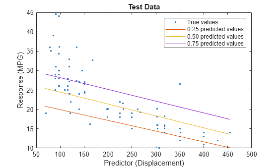
    The red line shows the predictions for the 0.25 quantile, the yellow line shows the predictions for the 0.50 quantile, and the purple line shows the predictions for the 0.75 quantile. The blue points indicate the true test data values.

    Notice that the quantile prediction lines do not cross each other.

    When training a quantile linear regression model, you can use a ridge (L2) regularization term to prevent quantile crossing.

    Load the carbig data set, which contains measurements of cars made in the 1970s and early 1980s. Create a table containing the predictor variables Acceleration, Cylinders, Displacement, and so on, as well as the response variable MPG.

    load carbig
    cars = table(Acceleration,Cylinders,Displacement, ...
        Horsepower,Model_Year,Weight,MPG);

    Remove rows of cars where the table has missing values.

    cars = rmmissing(cars);

    Partition the data into training and test sets using cvpartition. Use approximately 80% of the observations as training data, and 20% of the observations as test data.

    rng(0,"twister") % For reproducibility of the data partition
    c = cvpartition(height(cars),"Holdout",0.20);
    
    trainingIdx = training(c);
    carsTrain = cars(trainingIdx,:);
    
    testIdx = test(c);
    carsTest = cars(testIdx,:);

    Train a quantile linear regression model. Use the 0.25, 0.50, and 0.75 quantiles (that is, the lower quartile, median, and upper quartile). To improve the model fit, change the beta tolerance to 1e-6 instead of the default value 1e-4.

    Mdl = fitrqlinear(carsTrain,"MPG",Quantiles=[0.25 0.5 0.75], ...
        BetaTolerance=1e-6);

    Mdl is a RegressionQuantileLinear model object.

    Determine if the test data predictions for the quantiles in Mdl.Quantiles cross each other by using the predict object function of Mdl. The crossingIndicator output argument contains a value of 1 (true) for any observation with quantile predictions that cross.

    [~,crossingIndicator] = predict(Mdl,carsTest);
    sum(crossingIndicator)
    ans = 
    2
    

    In this example, two of the observations in carsTest have quantile predictions that cross each other.

    To prevent quantile crossing, specify the Lambda name-value argument in the call to fitrqlinear. Use a 0.1 ridge (L2) penalty term.

    newMdl = fitrqlinear(carsTrain,"MPG",Quantiles=[0.25 0.5 0.75], ...
        BetaTolerance=1e-6,Lambda=0.1);
    [predictedY,newCrossingIndicator] = predict(newMdl,carsTest);
    sum(newCrossingIndicator)
    ans = 
    0
    

    With regularization, the predictions for the test data set do not cross for any observations.

    Visualize the predictions returned by newMdl by using a scatter plot with a reference line. Plot the predicted values along the vertical axis and the true response values along the horizontal axis. Points on the reference line indicate correct predictions.

    plot(carsTest.MPG,predictedY(:,1),".")
    hold on
    plot(carsTest.MPG,predictedY(:,2),".")
    plot(carsTest.MPG,predictedY(:,3),".")
    plot(carsTest.MPG,carsTest.MPG)
    hold off
    xlabel("True MPG")
    ylabel("Predicted MPG")
    legend(["0.25 quantile values","0.50 quantile values", ...
        "0.75 quantile values","Reference line"], ...
        Location="southeast")
    title("Test Data")

    Figure contains an axes object. The axes object with title Test Data, xlabel True MPG, ylabel Predicted MPG contains 4 objects of type line. One or more of the lines displays its values using only markers These objects represent 0.25 quantile values, 0.50 quantile values, 0.75 quantile values, Reference line.

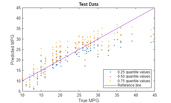
    Blue points correspond to the 0.25 quantile, red points correspond to the 0.50 quantile, and yellow points correspond to the 0.75 quantile.

    For a more in-depth example, see Regularize Quantile Regression Model to Prevent Quantile Crossing.

    Input Arguments

    collapse all

    Sample data used to train the model, specified as a table. Each row of Tbl corresponds to one observation, and each column corresponds to one predictor variable. Optionally, Tbl can contain one additional column for the response variable. Multicolumn variables and cell arrays other than cell arrays of character vectors are not allowed.

    • If Tbl contains the response variable, and you want to use all remaining variables in Tbl as predictors, then specify the response variable by using ResponseVarName.

    • If Tbl contains the response variable, and you want to use only a subset of the remaining variables in Tbl as predictors, then specify a formula by using formula.

    • If Tbl does not contain the response variable, then specify a response variable by using Y. The length of the response variable and the number of rows in Tbl must be equal.

    Response variable name, specified as the name of a variable in Tbl. The response variable must be a numeric vector.

    You must specify ResponseVarName as a character vector or string scalar. For example, if Tbl stores the response variable Y as Tbl.Y, then specify it as "Y". Otherwise, the software treats all columns of Tbl, including Y, as predictors when training the model.

    Data Types: char | string

    Explanatory model of the response variable and a subset of the predictor variables, specified as a character vector or string scalar in the form "Y~x1+x2+x3". In this form, Y represents the response variable, and x1, x2, and x3 represent the predictor variables.

    To specify a subset of variables in Tbl as predictors for training the model, use a formula. If you specify a formula, then the software does not use any variables in Tbl that do not appear in formula.

    The variable names in the formula must be both variable names in Tbl (Tbl.Properties.VariableNames) and valid MATLAB® identifiers. You can verify the variable names in Tbl by using the isvarname function. If the variable names are not valid, then you can convert them by using the matlab.lang.makeValidName function.

    Data Types: char | string

    Response data, specified as an n-dimensional numeric vector. The length of Y must be equal to the number of observations in X or Tbl.

    Data Types: single | double

    Predictor data used to train the model, specified as a numeric matrix.

    By default, the software treats each row of X as one observation, and each column as one predictor.

    The length of Y and the number of observations in X must be equal.

    To specify the names of the predictors in the order of their appearance in X, use the PredictorNames name-value argument.

    Note

    If you orient your predictor matrix so that observations correspond to columns and specify ObservationsIn="columns", then you might experience a significant reduction in computation time.

    Data Types: single | double

    Note

    The software treats NaN, empty character vector (''), empty string (""), <missing>, and <undefined> elements as missing values, and removes observations with any of these characteristics:

    • Missing value in the response

    • At least one missing value in a predictor observation

    • NaN value or 0 weight

    For economical memory usage, a best practice is to manually remove training observations that contain missing values before passing the data to fitrqlinear.

    Name-Value Arguments

    expand all

    Specify optional pairs of arguments as Name1=Value1,...,NameN=ValueN, where Name is the argument name and Value is the corresponding value. Name-value arguments must appear after other arguments, but the order of the pairs does not matter.

    Example: fitrqlinear(Tbl,"MPG",Quantiles=[0.25 0.5 0.75],Standardize=true) specifies to use the 0.25, 0.5, and 0.75 quantiles and to standardize the data before training.

    Linear Regression Options

    expand all

    Quantiles to use for training Mdl, specified as a vector of values in the range [0,1]. For each quantile q, the function fits a linear regression model that separates the bottom 100*q percent of training responses from the top 100*(1 – q) percent of training responses.

    You can find the estimated linear model coefficients and estimated bias term for each quantile in the Beta and Bias properties of Mdl, respectively.

    Example: Quantiles=[0.25 0.5 0.75]

    Data Types: single | double

    Initial coefficient estimates, specified as a p-by-q numeric matrix. p is the number of predictor variables after dummy variables are created for categorical variables (for more details, see CategoricalPredictors), and q is the number of quantiles (for more details, see Quantiles).

    By default, Beta is a matrix of 0 values.

    Data Types: single | double

    Initial intercept estimates, specified as a numeric vector of length q, where q is the number of quantiles (for more details, see Quantiles).

    By default, the initial bias for each quantile is the corresponding weighted quantile of the response.

    Data Types: single | double

    Flag to include the linear model intercept, specified as true or false.

    ValueDescription
    trueFor each quantile, the software includes the bias term b in the linear model, and then estimates it.
    falseThe software sets b = 0 during estimation.

    Example: FitBias=false

    Data Types: logical

    Regularization term strength, specified as "auto" or a nonnegative scalar. When the Lambda value is "auto", fitrqlinear uses 1/n as the regularization term strength, where n is the number of observations in X or Tbl.

    Example: Lambda=1e-4

    Data Types: single | double | char | string

    Predictor data observation dimension, specified as "rows" or "columns".

    Note

    If you orient your predictor matrix so that observations correspond to columns and specify ObservationsIn="columns", then you might experience a significant reduction in computation time. You cannot specify ObservationsIn="columns" for predictor data in a table.

    Example: ObservationsIn="columns"

    Data Types: char | string

    Objective function minimization technique for training, specified as "bfgs" or "lbfgs".

    • If X or Tbl contains 100 or fewer predictors, then the default value is "bfgs".

    • Otherwise, the default value is "lbfgs".

    Example: Solver="bfgs"

    Data Types: char | string

    Flag to standardize the predictor data, specified as a numeric or logical 0 (false) or 1 (true). If you set Standardize to true, then the software centers and scales each numeric predictor variable by the corresponding column mean and standard deviation. The software does not standardize categorical predictors.

    Example: Standardize=true

    Data Types: single | double | logical

    Convergence Control Options

    expand all

    Verbosity level, specified as a nonnegative integer. Verbose controls the amount of diagnostic information fitrqlinear displays at the command line.

    ValueDescription
    0fitrqlinear does not display diagnostic information.
    1fitrqlinear periodically displays and stores the value of the objective function, gradient magnitude, and other diagnostic information.
    Any other positive integerfitrqlinear displays and stores diagnostic information at each training process iteration.

    Example: Verbose=1

    Data Types: single | double

    Relative tolerance on the linear coefficients and the bias term (intercept) for each quantile, specified as a nonnegative scalar.

    Let Bt=[βtbt], that is, the vector of the coefficients and the bias term at iteration t of the training process. If BtBt1Bt2<BetaTolerance, then the training process terminates.

    Example: BetaTolerance=1e-6

    Data Types: single | double

    Absolute gradient tolerance for each quantile, specified as a nonnegative scalar.

    Let t be the gradient vector of the objective function with respect to the coefficients and bias term at iteration t of the training process. If t=max|t|<GradientTolerance, then the training process terminates.

    If you also specify BetaTolerance, then the training process terminates when fitrqlinear satisfies either stopping criterion.

    Example: GradientTolerance=eps

    Data Types: single | double

    Size of the history buffer for the Hessian approximation, specified as a positive integer. At each iteration, the software constructs the Hessian using statistics from the latest HessianHistorySize iterations.

    Example: HessianHistorySize=10

    Data Types: single | double

    Maximal number of iterations in the training process for each quantile, specified as a positive integer.

    Example: IterationLimit=1e7

    Data Types: single | double

    Other Regression Options

    expand all

    Categorical predictors list, specified as one of the values in this table. The descriptions assume that the predictor data has observations in rows and predictors in columns.

    ValueDescription
    Vector of positive integers

    Each entry in the vector is an index value indicating that the corresponding predictor is categorical. The index values are between 1 and p, where p is the number of predictors used to train the model.

    If fitrqlinear uses a subset of input variables as predictors, then the function indexes the predictors using only the subset. The CategoricalPredictors values do not count any response variable, observation weights variable, or other variable that the function does not use.

    Logical vector

    A true entry means that the corresponding predictor is categorical. The length of the vector is p.

    Character matrixEach row of the matrix is the name of a predictor variable. The names must match the entries in PredictorNames. Pad the names with extra blanks so each row of the character matrix has the same length.
    String array or cell array of character vectorsEach element in the array is the name of a predictor variable. The names must match the entries in PredictorNames.
    "all"All predictors are categorical.

    By default, if the predictor data is in a table (Tbl), fitrqlinear assumes that a variable is categorical if it is a logical vector, categorical vector, character array, string array, or cell array of character vectors. If the predictor data is a matrix (X), fitrqlinear assumes that all predictors are continuous. To identify any other predictors as categorical predictors, specify them by using the CategoricalPredictors name-value argument.

    For the identified categorical predictors, fitrqlinear creates dummy variables using two different schemes, depending on whether a categorical variable is unordered or ordered. For an unordered categorical variable, fitrqlinear creates one dummy variable for each level of the categorical variable. For an ordered categorical variable, fitrqlinear creates one less dummy variable than the number of categories. For details, see Automatic Creation of Dummy Variables.

    Example: CategoricalPredictors="all"

    Data Types: single | double | logical | char | string | cell

    Predictor variable names, specified as a string array of unique names or cell array of unique character vectors. The functionality of PredictorNames depends on the way you supply the training data.

    • If you supply X and Y, then you can use PredictorNames to assign names to the predictor variables in X.

      • The order of the names in PredictorNames must correspond to the predictor order in X. Assuming that X has the default orientation, with observations in rows and predictors in columns, PredictorNames{1} is the name of X(:,1), PredictorNames{2} is the name of X(:,2), and so on. Also, size(X,2) and numel(PredictorNames) must be equal.

      • By default, PredictorNames is {'x1','x2',...}.

    • If you supply Tbl, then you can use PredictorNames to choose which predictor variables to use in training. That is, fitrqlinear uses only the predictor variables in PredictorNames and the response variable during training.

      • PredictorNames must be a subset of Tbl.Properties.VariableNames and cannot include the name of the response variable.

      • By default, PredictorNames contains the names of all predictor variables.

      • A good practice is to specify the predictors for training using either PredictorNames or formula, but not both.

    Example: PredictorNames=["SepalLength","SepalWidth","PetalLength","PetalWidth"]

    Data Types: string | cell

    Response variable name, specified as a character vector or string scalar.

    • If you supply Y, then you can use ResponseName to specify a name for the response variable.

    • If you supply ResponseVarName or formula, then you cannot use ResponseName.

    Example: ResponseName="response"

    Data Types: char | string

    Function for transforming raw response values, specified as a function handle or function name. The default is "none", which means @(y)y, or no transformation. The function should accept a vector (the original response values) and return a vector of the same size (the transformed response values).

    Example: Suppose you create a function handle that applies an exponential transformation to an input vector by using myfunction = @(y)exp(y). Then, you can specify the response transformation as ResponseTransform=myfunction.

    Data Types: char | string | function_handle

    Since R2025a

    Option to perform computations in parallel using a parallel pool of workers, specified as one of these values:

    • false (0) — Run in serial on the MATLAB client.

    • true (1) — Use a parallel pool if one is open or if MATLAB can automatically create one. If a parallel pool is not available, run in serial on the MATLAB client.

    If you do not have a parallel pool open and automatic pool creation is enabled, MATLAB opens a pool using the default cluster profile. To use a parallel pool to run computations in MATLAB, you must have Parallel Computing Toolbox™. For more information, see Run MATLAB Functions with Automatic Parallel Support (Parallel Computing Toolbox).

    Tip

    Set UseParallel to true when the Quantiles value contains multiple quantiles. fitrqlinear performs all computations in serial when there is only one quantile.

    Example: UseParallel=true

    Data Types: single | double | logical | char | string

    Observation weights, specified as a nonnegative numeric vector or the name of a variable in Tbl. The software weights each observation in X or Tbl with the corresponding value in Weights. The length of Weights must equal the number of observations in X or Tbl.

    If you specify the input data as a table Tbl, then Weights can be the name of a variable in Tbl that contains a numeric vector. In this case, you must specify Weights as a character vector or string scalar. For example, if the weights vector W is stored as Tbl.W, then specify it as "W". Otherwise, the software treats all columns of Tbl, including W, as predictors when training the model.

    By default, Weights is ones(n,1), where n is the number of observations in X or Tbl.

    fitrqlinear normalizes the weights to sum to 1.

    Data Types: single | double | char | string

    Cross-Validation Options

    expand all

    Since R2025a

    Flag to train a cross-validated model, specified as "on" or "off".

    If you specify "on", then the software trains a cross-validated model with 10 folds.

    You can override this cross-validation setting using the CVPartition, Holdout, KFold, or Leaveout name-value argument. You can use only one cross-validation name-value argument at a time to create a cross-validated model.

    Alternatively, cross-validate later by passing Mdl to the crossval function.

    Example: CrossVal="on"

    Data Types: char | string

    Since R2025a

    Cross-validation partition, specified as a cvpartition object that specifies the type of cross-validation and the indexing for the training and validation sets.

    To create a cross-validated model, you can specify only one of these four name-value arguments: CVPartition, Holdout, KFold, or Leaveout.

    Example: Suppose you create a random partition for 5-fold cross-validation on 500 observations by using cvp = cvpartition(500,KFold=5). Then, you can specify the cross-validation partition by setting CVPartition=cvp.

    Since R2025a

    Fraction of the data used for holdout validation, specified as a scalar value in the range (0,1). If you specify Holdout=p, then the software completes these steps:

    1. Randomly select and reserve p*100% of the data as validation data, and train the model using the rest of the data.

    2. Store the compact trained model in the Trained property of the cross-validated model.

    To create a cross-validated model, you can specify only one of these four name-value arguments: CVPartition, Holdout, KFold, or Leaveout.

    Example: Holdout=0.1

    Data Types: double | single

    Since R2025a

    Number of folds to use in the cross-validated model, specified as a positive integer value greater than 1. If you specify KFold=k, then the software completes these steps:

    1. Randomly partition the data into k sets.

    2. For each set, reserve the set as validation data, and train the model using the other k – 1 sets.

    3. Store the k compact trained models in a k-by-1 cell vector in the Trained property of the cross-validated model.

    To create a cross-validated model, you can specify only one of these four name-value arguments: CVPartition, Holdout, KFold, or Leaveout.

    Example: KFold=5

    Data Types: single | double

    Since R2025a

    Leave-one-out cross-validation flag, specified as "on" or "off". If you specify Leaveout="on", then for each of the n observations (where n is the number of observations, excluding missing observations, specified in the NumObservations property of the model), the software completes these steps:

    1. Reserve the one observation as validation data, and train the model using the other n – 1 observations.

    2. Store the n compact trained models in an n-by-1 cell vector in the Trained property of the cross-validated model.

    To create a cross-validated model, you can specify only one of these four name-value arguments: CVPartition, Holdout, KFold, or Leaveout.

    Example: Leaveout="on"

    Data Types: char | string

    Note

    You cannot use any cross-validation name-value argument together with the OptimizeHyperparameters name-value argument. You can modify the cross-validation for OptimizeHyperparameters only by using the HyperparameterOptimizationOptions name-value argument.

    Hyperparameter Optimization Options

    expand all

    Since R2025a

    Parameters to optimize, specified as one of the following:

    • "none" — Do not optimize.

    • "auto" — Use ["Lambda","Standardize"].

    • "all" — Optimize all eligible parameters.

    • String array or cell array of eligible parameter names.

    • Vector of optimizableVariable objects, typically the output of hyperparameters.

    You can optimize hyperparameters only when creating a quantile regression model with one quantile (that is, the Quantiles name-value argument has one element).

    The optimization attempts to minimize the cross-validation loss (error) for fitrqlinear by varying the parameters. To control the cross-validation type and other aspects of the optimization, use the HyperparameterOptimizationOptions name-value argument. When you use HyperparameterOptimizationOptions, you can use the (compact) model size instead of the cross-validation loss as the optimization objective by setting the ConstraintType and ConstraintBounds options.

    Note

    The values of OptimizeHyperparameters override any values you specify using other name-value arguments. For example, setting OptimizeHyperparameters to "auto" causes fitrqlinear to optimize hyperparameters corresponding to the "auto" option and to ignore any specified values for the hyperparameters.

    The eligible parameters for fitrqlinear are:

    • Lambdafitrqlinear optimizes Lambda over log-scaled values in the range [1e-5/NumObservations,1e5/NumObservations].

    • Standardizefitrqlinear optimizes Standardize over the two values [true,false].

    Set nondefault parameters by passing a vector of optimizableVariable objects that have nondefault values. For example:

    load carsmall
    params = hyperparameters("fitrqlinear",[Horsepower,Weight],MPG);
    params(1).Range = [1e-3,2e4];

    Pass params as the value of OptimizeHyperparameters.

    By default, the iterative display appears at the command line, and plots appear according to the number of hyperparameters in the optimization. For the optimization and plots, the objective function is log(1 + cross-validation loss). To control the iterative display, set the Verbose option of the HyperparameterOptimizationOptions name-value argument. To control the plots, set the ShowPlots option of the HyperparameterOptimizationOptions name-value argument.

    Example: OptimizeHyperparameters="auto"

    Since R2025a

    Options for optimization, specified as a HyperparameterOptimizationOptions object or a structure. This argument modifies the effect of the OptimizeHyperparameters name-value argument. If you specify HyperparameterOptimizationOptions, you must also specify OptimizeHyperparameters. All the options listed in the following table are optional. However, you must set ConstraintBounds and ConstraintType to return AggregateOptimizationResults. The options that you can set in a structure are the same as those in the HyperparameterOptimizationOptions object.

    OptionValuesDefault
    Optimizer
    • "bayesopt" — Use Bayesian optimization. Internally, this setting calls bayesopt.

    • "gridsearch" — Use grid search with NumGridDivisions values per dimension. "gridsearch" searches in a random order, using uniform sampling without replacement from the grid. After optimization, you can get a table in grid order by using the command sortrows(Mdl.HyperparameterOptimizationResults).

    • "randomsearch" — Search at random among MaxObjectiveEvaluations points.

    "bayesopt"
    ConstraintBounds

    Constraint bounds for N optimization problems, specified as an N-by-2 numeric matrix or []. The columns of ConstraintBounds contain the lower and upper bound values of the optimization problems. If you specify ConstraintBounds as a numeric vector, the software assigns the values to the second column of ConstraintBounds, and zeros to the first column. If you specify ConstraintBounds, you must also specify ConstraintType.

    []
    ConstraintTarget

    Constraint target for the optimization problems, specified as "matlab" or "coder". If ConstraintBounds and ConstraintType are [] and you set ConstraintTarget, then the software sets ConstraintTarget to []. The values of ConstraintTarget and ConstraintType determine the objective and constraint functions. For more information, see HyperparameterOptimizationOptions.

    If you specify ConstraintBounds and ConstraintType, then the default value is "matlab". Otherwise, the default value is [].
    ConstraintType

    Constraint type for the optimization problems, specified as "size" or "loss". If you specify ConstraintType, you must also specify ConstraintBounds. The values of ConstraintTarget and ConstraintType determine the objective and constraint functions. For more information, see HyperparameterOptimizationOptions.

    []
    AcquisitionFunctionName

    Type of acquisition function:

    • "expected-improvement-per-second-plus"

    • "expected-improvement"

    • "expected-improvement-plus"

    • "expected-improvement-per-second"

    • "lower-confidence-bound"

    • "probability-of-improvement"

    Acquisition functions whose names include per-second do not yield reproducible results, because the optimization depends on the run time of the objective function. Acquisition functions whose names include plus modify their behavior when they overexploit an area. For more details, see Acquisition Function Types.

    "expected-improvement-per-second-plus"
    MaxObjectiveEvaluationsMaximum number of objective function evaluations. If you specify multiple optimization problems using ConstraintBounds, the value of MaxObjectiveEvaluations applies to each optimization problem individually.30 for "bayesopt" and "randomsearch", and the entire grid for "gridsearch"
    MaxTime

    Time limit for the optimization, specified as a nonnegative real scalar. The time limit is in seconds, as measured by tic and toc. The software performs at least one optimization iteration, regardless of the value of MaxTime. The run time can exceed MaxTime because MaxTime does not interrupt function evaluations. If you specify multiple optimization problems using ConstraintBounds, the time limit applies to each optimization problem individually.

    Inf
    NumGridDivisionsFor Optimizer="gridsearch", the number of values in each dimension. The value can be a vector of positive integers giving the number of values for each dimension, or a scalar that applies to all dimensions. The software ignores this option for categorical variables.10
    ShowPlotsLogical value indicating whether to show plots of the optimization progress. If this option is true, the software plots the best observed objective function value against the iteration number. If you use Bayesian optimization (Optimizer="bayesopt"), the software also plots the best estimated objective function value. The best observed objective function values and best estimated objective function values correspond to the values in the BestSoFar (observed) and BestSoFar (estim.) columns of the iterative display, respectively. You can find these values in the properties ObjectiveMinimumTrace and EstimatedObjectiveMinimumTrace of Mdl.HyperparameterOptimizationResults. If the problem includes one or two optimization parameters for Bayesian optimization, then ShowPlots also plots a model of the objective function against the parameters.true
    SaveIntermediateResultsLogical value indicating whether to save the optimization results. If this option is true, the software overwrites a workspace variable named "BayesoptResults" at each iteration. The variable is a BayesianOptimization object. If you specify multiple optimization problems using ConstraintBounds, the workspace variable is an AggregateBayesianOptimization object named "AggregateBayesoptResults".false
    Verbose

    Display level at the command line:

    • 0 — No iterative display

    • 1 — Iterative display

    • 2 — Iterative display with additional information

    For details, see the bayesopt Verbose name-value argument and the example Optimize Classifier Fit Using Bayesian Optimization.

    1
    UseParallelLogical value indicating whether to run the Bayesian optimization in parallel, which requires Parallel Computing Toolbox. Due to the nonreproducibility of parallel timing, parallel Bayesian optimization does not necessarily yield reproducible results. For details, see Parallel Bayesian Optimization.false
    Repartition

    Logical value indicating whether to repartition the cross-validation at every iteration. If this option is false, the optimizer uses a single partition for the optimization.

    A value of true usually gives the most robust results because this setting takes partitioning noise into account. However, for optimal results, true requires at least twice as many function evaluations.

    false
    Specify only one of the following three options.
    CVPartitioncvpartition object created by cvpartitionKFold=5 if you do not specify a cross-validation option
    HoldoutScalar in the range (0,1) representing the holdout fraction
    KFoldInteger greater than 1

    Example: HyperparameterOptimizationOptions=struct(UseParallel=true)

    Output Arguments

    collapse all

    Trained quantile linear regression model, returned as a RegressionQuantileLinear object, a RegressionPartitionedQuantileModel object, or a cell array of model objects.

    • If you set any of the name-value arguments CrossVal, CVPartition, Holdout, KFold, or Leaveout, then Mdl is a RegressionPartitionedQuantileModel object.

    • If you specify OptimizeHyperparameters and set the ConstraintType and ConstraintBounds options of HyperparameterOptimizationOptions, then Mdl is an N-by-1 cell array of model objects, where N is equal to the number of rows in ConstraintBounds. If none of the optimization problems yields a feasible model, then each cell array value is [].

    • Otherwise, Mdl is a RegressionQuantileLinear model object.

    To reference properties of a model object, use dot notation.

    Since R2025a

    Aggregate optimization results for multiple optimization problems, returned as an AggregateBayesianOptimization object. To return AggregateOptimizationResults, you must specify OptimizeHyperparameters and HyperparameterOptimizationOptions. You must also specify the ConstraintType and ConstraintBounds options of HyperparameterOptimizationOptions. For an example that shows how to produce this output, see Hyperparameter Optimization with Multiple Constraint Bounds.

    Tips

    Extended Capabilities

    expand all

    Version History

    Introduced in R2024b

    expand all