MultinomialRegression

Multinomial regression model

Since R2023a

Description

MultinomialRegression is a fitted multinomial regression model object. A multinomial regression model describes the relationship between predictors and a response that has a finite set of values.

Use the properties of a MultinomialRegression object to investigate a fitted multinomial regression model. The object properties include information about coefficient estimates, summary statistics, and the data used to fit the model. Use the object functions to predict responses, and to evaluate and visualize the multinomial regression model.

Creation

Create a MultinomialRegression model object with specified parameter values by using fitmnr.

Properties

Coefficient Estimates

ClassNames — Names of response variable categories

categorical array | character array | logical vector | numeric vector | cell array of character vectors

This property is read-only.

Names of the response variable categories used to fit the multinomial regression model, specified as a k-by-1 categorical array, character array, logical vector, numeric vector, or cell array of character vectors. k is the number of response categories. ClassNames has the same data type as the response category labels. Note that the software treats string arrays as cell arrays of character vectors. The ClassNames property is set by the fitmnr input argument Y or Tbl when you create the model object.

Data Types: single | double | logical | char | cell | categorical

CoefficientCovariance — Covariance matrix for model coefficients

(p+1)-by-(p+1) matrix of numeric values

This property is read-only.

Covariance matrix for model coefficients, specified as a (p+1)-by-(p+1) matrix of numeric values. p is the number of predictor variables.

For details, see Coefficient Standard Errors and Confidence Intervals.

Data Types: single | double

CoefficientNames — Coefficient names

cell array of character vectors

This property is read-only.

Coefficient names, specified as a cell array of character vectors, each containing the name of the corresponding coefficient. Each coefficient name is the name of a response category appended to the name of a predictor or intercept. This property is set by the fitmnr input argument Tbl or name-value argument PredictorNames when you create the model object.

Data Types: cell

Coefficients — Coefficient values

table

This property is read-only.

Coefficient values, specified as a table that contains one row for each coefficient and these columns:

• Value — Estimated coefficient value

• SE — Standard error of the estimate

• tStat — t-statistic for a two-sided test with the null hypothesis that the coefficient is zero

• pValue — p-value for the t-statistic

Use coefTest or testDeviance to perform other tests on the coefficients. Use coefCI to find the confidence intervals of the coefficient estimates.

Data Types: table

IncludeClassInteractions — Indicator for interaction between response categories and coefficients

true or 1 | false or 0

This property is read-only.

Indicator for an interaction between response categories and coefficients, specified as a numeric or logical 1 (true) or 0 (false). This property is set by the fitmnr name-value argument IncludeClassInteractions when you create the model object.

Data Types: logical

Link — Link function

'logit' | 'probit' | 'comploglog' | 'loglog'

This property is read-only.

Link function to use for ordinal and hierarchical models, specified as 'logit', 'probit', 'comploglog', or 'loglog'. For nominal models, Link is always 'logit'. This property is set by the fitmnr name-value argument Link when you create the model object.

Data Types: char

ModelType — Type of model

'nominal' | 'ordinal' | 'hierarchical'

This property is read-only.

Type of model, specified as 'nominal', 'ordinal', or 'hierarchical'. This property is set by the fitmnr name-value argument ModelType when you create the model object.

Data Types: char

NumCoefficients — Number of model coefficients

positive integer

This property is read-only.

Number of model coefficients, specified as a positive integer.

Data Types: double

Summary Statistics

Deviance — Deviance of fit

numeric value

This property is read-only.

Deviance of the fit, specified as a numeric value. The deviance is useful for comparing two models when one model is a special case of the other model. The difference between the deviance of the two models has a chi-square distribution with degrees of freedom equal to the difference in the number of estimated parameters between the two models. For more information, see Deviance.

Data Types: single | double

DFE — Degrees of freedom for error

positive integer

This property is read-only.

Degrees of freedom for the error (residuals), specified as a positive integer. For nominal and ordinal models, DFE is given by

$$DFE=n*(k-1)-N,$$

where n is the number of observations, k is the number of response categories, and N is the number of model coefficients. For hierarchical models, DFE is given by

$$DFE=n-N,$$

when IncludeClassInteractions is false. When IncludeClassInteractions is true, DFE for a hierarchical model is given by

$$DFE=\left({\displaystyle \sum _{i=1}^{k-1}{n}_i}\right)-N,$$

where n_i is the number of observations corresponding to the ith response category and above.

Data Types: double

Dispersion — Variance

numeric scalar

This property is read-only.

Variance, specified as a numeric scalar. If you set the fitmnr EstimateDispersion name-value argument to true when you create the model object, the function estimates the standard error as the Dispersion value. Otherwise, fitmnr assigns the default theoretical value of 1 to Dispersion.

Data Types: single | double

EstimateDispersion — Indicator for whether dispersion is estimated

false | true

This property is read-only.

Indicator for whether dispersion is estimated, specified as a logical false or true. This property is set by the fitmnr EstimateDispersion name-value argument when you create the model object.

Data Types: single | double | logical

Fitted — Fitted response values based on input data

categorical array | character array | logical vector | numeric vector | cell array of character vectors

This property is read-only.

Fitted (predicted) response values based on the input data, specified as an n-by-1 categorical array, character array, logical vector, numeric vector, or cell array of character vectors. n is the number of observations in the input data. Fitted has the same data type as the response category labels. Note that the software treats string arrays as cell arrays of character vectors. Use predict to compute the predictions for other predictor values, or to compute the confidence bounds on Fitted.

Data Types: single | double | logical | char | cell | categorical

LogLikelihood — Loglikelihood of fitted model

numeric value

This property is read-only.

Loglikelihood of the fitted model, specified as a numeric value, based on the assumption that each response value follows a multinomial distribution. When you create the model object, fitmnr calculates the loglikelihood of the model by taking the sum of the log probabilities for the response data.

Data Types: single | double

ModelCriterion — Criterion for model comparison

structure

This property is read-only.

Criterion for model comparison, specified as a structure with these fields:

• AIC — Akaike information criterion. AIC = –2*lnL + 2*m, where lnL is the loglikelihood and m is the number of estimated parameters.

• AICc — Akaike information criterion corrected for the sample size. AICc = AIC + (2*m*(m + 1))/(n – m – 1), where n is the number of observations.

• BIC — Bayesian information criterion. BIC = –2*lnL + m*ln(n).

• CAIC — Consistent Akaike information criterion. CAIC = –2*lnL + m*(ln(n) + 1).

Information criteria are model selection tools you can use to compare multiple models that are fit to the same data. These criteria are likelihood-based measures of model fit that include a penalty for complexity (specifically, the number of parameters). Different information criteria are distinguished by the form of the penalty.

When you compare multiple models, the model with the lowest information criterion value is the best-fitting model. The best-fitting model can vary depending on the criterion used for model comparison.

Data Types: struct

Residuals — Residuals for fitted model

table

This property is read-only.

Residuals for the fitted model, specified as a table in which each variable contains one row for each observation and one column for each response class.

Column	Description
Raw	Raw residuals. Observed minus fitted values, $$r_{ij}=y_{ij}-{\widehat{\pi }}_{ij}*m_i,\{\begin{array}{c}i=1,\cdots ,n\\ j=1,\cdots ,N\end{array}.$$ yij is a logical scalar indicating whether the ith data point is in the jth response category $${\widehat{\pi }}_{ij}$$ is the predicted probability of the ith data point being in the jth response category mi is the corresponding sample size for observation i n and N are the number of data points and response categories, respectively
Pearson	Raw residuals divided by the root mean squared error (RMSE)
Deviance	Deviance residuals given by the formula $$r{d}_i=2*{\displaystyle {\sum }_j^k{y}_{ij}*\log \left(\frac{y_{ij}}{{\widehat{\pi }}_{ij}*m_i}\right)},i=1,\cdots ,n.$$

Rows not used in the fit because of missing values contain NaN values. To inspect missing values, see ObservationInfo.

Use plotResiduals to create a plot of the residuals. For details, see Residuals.

Data Types: table

Rsquared — Pseudo R-squared values for the fitted model

structure

This property is read-only.

Pseudo R-squared values for the fitted model, specified as a structure. Each field of Rsquared contains a pseudo R-squared value calculated with a different formula [1].

Field	Description
'Ordinary'	The ordinary pseudo R-squared value is $$R^2=1-\frac{\ln (L_{Full})}{\ln (L_{Null})},$$ where $$L_{Full}$$ is the loglikelihood of the fitted model and $$L_{Null}$$ is the loglikelihood of a model with no predictors.
'Adjusted'	The adjusted pseudo R-squared value is $$R^2=1-\frac{\ln (L_{Full})-K}{\ln (L_{Null})},$$ where K is the number of model coefficients in $$L_{Full}$$.

Data Types: struct

Input Data

Formula — Regression model

LinearFormula object

This property is read-only.

Regression model, specified as a LinearFormula object. This property is set by the fitmnr input argument Formula when you create the model object.

NumObservations — Number of observations

positive integer

This property is read-only.

Number of observations used by the fitting algorithm to fit the model, specified as a positive integer. NumObservations is the number of observations supplied in the original table or matrix, minus any rows with missing values.

Data Types: double

NumPredictors — Number of predictor variables

positive integer

This property is read-only.

Number of predictor variables used by the fitting algorithm to fit the model, specified as a positive integer.

Data Types: double

NumVariables — Number of variables

positive integer

This property is read-only.

Number of variables in the input data, specified as a positive integer. NumVariables includes any variables that are not used as predictors or as the response to fit the model.

Data Types: double

ObservationInfo — Observation information

n-by-3 table

This property is read-only.

Observation information, specified as an n-by-3 table containing the following columns, where n is the number of observations.

Column	Description
Weights	Observation weights, specified as a numeric value. The default value is 1.
Missing	Indicator of missing observations, specified as a logical value. The value is true if the observation is missing.
Subset	Indicator of whether fitmnr uses the observation, specified as a logical value. The value is true if the observation is not missing, meaning fitmnr uses the observation.

Data Types: table

ObservationNames — Observation names

cell array of character vectors

This property is read-only.

Observation names, specified as a cell array of character vectors containing the names of the observations used in the fit.

• If the fit is based on a table or dataset containing observation names, the ObservationNames property contains those names.

• Otherwise, ObservationNames is an empty cell array.

This property is set by the fitmnr input argument Tbl when you create the model object and assign row names to Tbl.

Data Types: cell

PredictorNames — Names of predictors used to fit model

cell array of character vectors

This property is read-only.

Names of the predictors used to fit the model, specified as a cell array of character vectors. This property is set by one of the following fitmnr arguments when you create the model object:

• Tbl input argument

• X input argument together with the PredictorNames name-value argument

Data Types: cell

ResponseName — Response variable name

character vector

This property is read-only.

Response variable name, specified as a character vector. This property is set by one of the following fitmnr arguments when you create the model object:

• ResponseName name-value argument

• Tbl input argument together with the ResponseVarName input argument

• Tbl input argument together with the Formula input argument

Data Types: char

VariableInfo — Information about variables

table

This property is read-only.

Information about the variables contained in the Variables property, specified as a table with one row for each variable and the following columns.

Column	Description
Class	Variable class, specified as a cell array of character vectors, such as 'double' and 'categorical'
Range	Variable range, specified as a cell array of vectors Continuous variable — Two-element vector [min,max], the minimum and maximum values Categorical variable — Vector of distinct variable values
InModel	Indicator of which variables are in the fitted model, specified as a logical vector. The value is true if the model includes the variable.
IsCategorical	Indicator of categorical variables, specified as a logical vector. The value is true if the variable is categorical.

VariableInfo also includes any variables that are not used as predictors or as the response to fit the model.

Data Types: table

VariableNames — Names of variables

cell array of character vectors

This property is read-only.

Names of the variables, specified as a cell array of character vectors. Elements of this property are set by one of the following fitmnr arguments when you create the model object:

• The Tbl input argument specifies the names of the predictor variables, response, and unused variables.

• The PredictorNames name-value argument specifies the names of the predictor variables.

• The ResponseVarName name-value argument specifies the name of the response variable.

VariableNames also includes any variables that are not used as predictors or as the response to fit the model.

Data Types: cell

Variables — Input data

table

This property is read-only.

Input data, specified as a table. Variables contains both predictor and response values. Elements of this property are set by one of the following fitmnr arguments when you create the model object:

• If you specify X, then Variables contains all variables in the columns of X.

• If you specify Tbl, then Variables contains all variables in Tbl, including variables not used as predictor or response data to fit the model.

• If you specify Y, then Variables also contains the response data in Y.

Data Types: table

Object Functions

coefCI	Confidence intervals for coefficient estimates of multinomial regression model
coefTest	Linear hypothesis test on multinomial regression model coefficients
feval	Predict responses of multinomial regression model using one input for each predictor
partialDependence	Compute partial dependence
plotPartialDependence	Create partial dependence plot (PDP) and individual conditional expectation (ICE) plots
plotResiduals	Plot residuals of multinomial regression model
plotSlice	Plot of slices through fitted multinomial regression surface
predict	Predict responses of multinomial regression model
random	Generate random responses from fitted multinomial regression model
testDeviance	Deviance test for multinomial regression model

Examples

Analyze Nominal Model Coefficients

Load the fisheriris sample data set.

load fisheriris

The column vector species contains iris flowers of three different species: setosa, versicolor, virginica. The matrix meas contains four types of measurements for the flower: the length and width of sepals and petals in centimeters.

Fit a multinomial regression model to predict the iris flower species using the measurements. Display the results of the fit using the Coefficients property of the fitted model.

MnrModel = fitmnr(meas,species);
MnrModel.Coefficients

ans=10×4 table
                               Value       SE       tStat       pValue  
                              _______    ______    _______    __________

    (Intercept_setosa)         1969.2    12.404     158.76             0
    x1_setosa                   657.5    3.5783     183.75             0
    x2_setosa                 -554.54     3.176     -174.6             0
    x3_setosa                 -503.76    3.5403    -142.29             0
    x4_setosa                 -2694.2    7.1203    -378.39             0
    (Intercept_versicolor)     42.638    5.2719     8.0878    6.0776e-16
    x1_versicolor              2.4652    1.1228     2.1956      0.028124
    x2_versicolor              6.6809    1.4789     4.5176    6.2559e-06
    x3_versicolor             -9.4294    1.2934    -7.2906     3.086e-13
    x4_versicolor             -18.286    2.0967    -8.7214    2.7476e-18

MnrModel is a multinomial regression model object that contains the results of fitting a nominal multinomial regression model to the data. The Coefficients property contains coefficient statistics for each predictor in meas. The small p-values in the column pValue indicate that all coefficients are statistically significant at the 95% confidence level. fitmnr sorts the categories in species in order of their first appearance. The last category is the default reference category.

To display the sorted names of the response variable categories, use the ClassNames property of MnrModel.

MnrModel.ClassNames

ans = 3x1 cell
    {'setosa'    }
    {'versicolor'}
    {'virginica' }

The output shows that the last category, 'virginica', is the reference category by default.

To get 95% confidence intervals for the fitted coefficient estimates, call the object function coefCI.

coefCI(MnrModel)

ans = 10×2
103 ×

    1.9448    1.9936
    0.6505    0.6645
   -0.5608   -0.5483
   -0.5107   -0.4968
   -2.7083   -2.6802
    0.0323    0.0530
    0.0003    0.0047
    0.0038    0.0096
   -0.0120   -0.0069
   -0.0224   -0.0142

The output shows 95% confidence intervals for the 10 coefficients in the Value column of the Coefficients table. None of the confidence intervals cross zero, confirming that all coefficients affect the log odds at the 95% confidence level.

Predict Response Categories

Load the fisheriris sample data set.

load fisheriris

The column vector species contains three iris flowers species: setosa, versicolor, and virginica. The matrix meas contains four types of measurements for the flower: the length and width of sepals and petals in centimeters.

Divide the species and measurement data into training and test data by using the cvpartition function. Get the indices of the training data rows by using the training function.

n = length(species);
partition = cvpartition(n,'Holdout',0.05);
idx_train = training(partition);

Create training data by using the indices of the training data rows to create a matrix of measurements and a vector of species labels.

meastrain = meas(idx_train,:);
speciestrain = species(idx_train,:);

Fit a multinomial regression model using the training data.

mdl = fitmnr(meastrain,speciestrain)

mdl = 
Multinomial regression with nominal responses

                               Value       SE       tStat        pValue  
                              _______    ______    ________    __________

    (Intercept_setosa)         86.305    12.541      6.8817    5.9158e-12
    x1_setosa                 -1.0728    3.5795    -0.29971        0.7644
    x2_setosa                  23.846    3.1238      7.6336    2.2835e-14
    x3_setosa                 -27.289    3.5009      -7.795    6.4409e-15
    x4_setosa                  -59.58    7.0214     -8.4855    2.1472e-17
    (Intercept_versicolor)     42.637    5.2214      8.1659    3.1906e-16
    x1_versicolor              2.4652    1.1263      2.1887      0.028619
    x2_versicolor              6.6808     1.474      4.5325     5.829e-06
    x3_versicolor             -9.4292    1.2946     -7.2837     3.248e-13
    x4_versicolor             -18.286    2.0833     -8.7775     1.671e-18


143 observations, 276 error degrees of freedom
Dispersion: 1
Chi^2-statistic vs. constant model: 302.0378, p-value = 1.5168e-60

mdl is a multinomial regression model object that contains the results of fitting a nominal multinomial regression model to the data. The table output shows coefficient statistics for each predictor in meas. By default, fitmnr uses virginica as the reference category.

Get the indices of the test data rows by using the test function. Create test data by using the indices of the test data rows to create a matrix of measurements and a vector of species labels.

idx_test = test(partition);
meastest = meas(idx_test,:);
speciestest = species(idx_test,:);

Predict the iris species for the measurements in meastest.

speciespredict = predict(mdl,meastest)

speciespredict = 7x1 cell
    {'setosa'    }
    {'setosa'    }
    {'setosa'    }
    {'setosa'    }
    {'setosa'    }
    {'versicolor'}
    {'versicolor'}

Compare the predictions in speciespredict with the category names in speciestest.

speciestest

speciestest = 7x1 cell
    {'setosa'    }
    {'setosa'    }
    {'setosa'    }
    {'setosa'    }
    {'setosa'    }
    {'versicolor'}
    {'versicolor'}

The output shows that the model accurately predicts the iris species for the measurements in meastest.

Plot Engine Cylinder Probabilities

Load the carbig sample data set.

load carbig;

The vectors Acceleration and Displacement contain data for car acceleration and displacement, respectively. The vector Cylinders contains data for the number of cylinders in each car engine.

Fit an ordinal multinomial regression model using Acceleration and Displacement as predictor variables and Cylinders as the response variable.

MnrModel = fitmnr([Acceleration,Displacement],Cylinders,Model="ordinal",...
    PredictorNames=["Acceleration" "Displacement"])

MnrModel = 
Multinomial regression with ordinal responses

                       Value         SE        tStat       pValue  
                     _________    ________    _______    __________

    (Intercept_3)       11.949      3.1817     3.7555    0.00017299
    (Intercept_4)        27.08      4.9481     5.4727    4.4321e-08
    (Intercept_5)       27.528      4.9738     5.5346    3.1195e-08
    (Intercept_6)       45.346      7.8292     5.7919    6.9593e-09
    Acceleration     -0.063533      0.1041    -0.6103       0.54167
    Displacement      -0.16731    0.027885         -6    1.9726e-09


406 observations, 1618 error degrees of freedom
Dispersion: 1
Chi^2-statistic vs. constant model: 786.5846, p-value = 1.5679e-171

MnrModel is a multinomial regression model object that contains the results of fitting an ordinal multinomial regression model to the data. The table output shows coefficient statistics for each predictor variable. The p-values in the column pValue indicate that there is not enough evidence to conclude that the coefficient for the Acceleration term is statistically significant. However, enough evidence exists to conclude that Displacement has a statistically significant effect at the 99% confidence level.

Display the possible quantities for car engine cylinders using the ClassNames property.

MnrModel.ClassNames

ans = 5×1

     3
     4
     5
     6
     8

The last category in the output is the default reference category. The output shows that the reference category corresponds to cars with eight-cylinder engines.

Use plotSlice to plot stacked histograms of the probabilities of a car having each number of cylinders as the value of the predictor variable Displacement changes. By default, plotSlice fixes the value of Acceleration at its training data mean.

plotSlice(MnrModel,"stackedhist",PredictorToVary="Displacement")
hold on
lgd = legend;
title(lgd, "Number of cylinders");

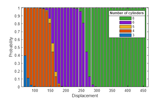
The plot shows that the probability of a car having more cylinders increases as the car displacement increases, which is consistent with the small p-value for the Displacement model term.

Analyze Effect of Car Displacement on Reference Category Probability

Load the carbig sample data set.

load carbig;

The vectors Acceleration and Displacement contain data for car acceleration and displacement, respectively. The vector Cylinders contains data for the number of cylinders in each car engine.

Fit an ordinal multinomial regression model using Acceleration and Displacement as predictor variables and Cylinders as the response variable.

MnrModel = fitmnr([Acceleration,Displacement],Cylinders,Model="ordinal",...
    PredictorNames=["Acceleration" "Displacement"])

MnrModel = 
Multinomial regression with ordinal responses

                       Value         SE        tStat       pValue  
                     _________    ________    _______    __________

    (Intercept_3)       11.949      3.1817     3.7555    0.00017299
    (Intercept_4)        27.08      4.9481     5.4727    4.4321e-08
    (Intercept_5)       27.528      4.9738     5.5346    3.1195e-08
    (Intercept_6)       45.346      7.8292     5.7919    6.9593e-09
    Acceleration     -0.063533      0.1041    -0.6103       0.54167
    Displacement      -0.16731    0.027885         -6    1.9726e-09


406 observations, 1618 error degrees of freedom
Dispersion: 1
Chi^2-statistic vs. constant model: 786.5846, p-value = 1.5679e-171

MnrModel is a multinomial regression model object that contains the results of fitting an ordinal multinomial regression model to the data. The table output shows coefficient statistics for each of the predictor variable. The p-values in the column pValue indicate that there is not enough evidence to conclude that the coefficient for the Acceleration term is statistically significant. However, enough evidence exists to conclude that Displacement has a statistically significant effect at the 99% confidence level.

Display the possible quantities for car engine cylinders using the ClassNames property.

MnrModel.ClassNames

ans = 5×1

     3
     4
     5
     6
     8

The reference category corresponds to cars with eight-cylinder engines.

Plot the partial dependence of the reference category probability on the Displacement predictor by using the plotPartialDependence object function.

plotPartialDependence(MnrModel,2,8)

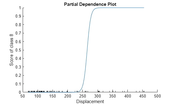
The plot shows that the probability of a car being in the reference category increases sharply when the value of Displacement reaches approximately 250.

More About

Deviance

Deviance is a generalization of the residual sum of squares. It measures the goodness of fit compared to a saturated model.

The deviance of a model M₁ is twice the difference between the loglikelihood of the model M₁ and the saturated model M_s. A saturated model is a model with the maximum number of parameters that you can estimate.

For example, if you have n observations with potentially different response values y_i, i = 1, 2, ..., n, then you can define a saturated model (with n parameters) that perfectly predicts the responses. Let L(b,y) denote the maximum value of the likelihood function for a model with the parameters b. Then the deviance of the model M₁ is

$$-2\left(\log L\left(b_1,y\right)-\log L\left(b_S,y\right)\right),$$

where b₁ and b_s contain the estimated parameters for the model M₁ and the saturated model, respectively. The deviance has a chi-square distribution with n – p degrees of freedom, where n is the number of parameters in the saturated model and p is the number of parameters in the model M₁.

Assume you have two different multinomial regression models M₁ and M₂, and M₁ has a subset of the terms in M₂. You can evaluate the fit of the models by comparing the deviances D₁ and D₂ of the two models. The difference of the deviances is

$$\begin{array}{l}D=D_2-D_1=-2\left(\log L\left(b_2,y\right)-\log L\left(b_S,y\right)\right)+2\left(\log L\left(b_1,y\right)-\log L\left(b_S,y\right)\right)\\ =-2\left(\log L\left(b_2,y\right)-\log L\left(b_1,y\right)\right).\end{array}$$

Asymptotically, the difference D has a chi-square distribution with degrees of freedom v equal to the difference in the number of parameters estimated in M₁ and M₂. You can obtain the p-value for this test by using 1 – chi2cdf(D,v,"upper").

Typically, you examine D using a model M₂ with a constant term and no predictors. Therefore, D has a chi-square distribution with p – 1 degrees of freedom. If the dispersion is estimated, the difference divided by the estimated dispersion has an F distribution with p – 1 numerator degrees of freedom and n – p denominator degrees of freedom.

References

[1] Allison, P. D. "Measures of Fit for Logistic Regression." Statistical Horizons LLC and the University of Pennsylvania, 2014.

[2] McCullagh, P., and J. A. Nelder. Generalized Linear Models. New York: Chapman & Hall, 1990.

[3] Long, J. S. Regression Models for Categorical and Limited Dependent Variables. Sage Publications, 1997.

[4] Dobson, A. J., and A. G. Barnett. An Introduction to Generalized Linear Models. Chapman and Hall/CRC. Taylor & Francis Group, 2008.

Version History

Introduced in R2023a