Fixed Effects Panel Model with Concurrent Correlation

Open Live Script

This example shows how to perform panel data analysis using mvregress. First, a fixed effects model with concurrent correlation is fit by ordinary least squares (OLS) to some panel data. Then, the estimated error covariance matrix is used to get panel corrected standard errors for the regression coefficients.

Load Sample Data

Load the sample panel data.

load panelTbl

The panelTbl data set contains yearly observations on eight cities for 6 years. This is simulated data.

Define Variables

The first variable, Growth, measures economic growth (the response variable). The second and third variables are city and year indicators, respectively. The last variable, Employ, measures employment (the predictor variable).

y = panelTbl.Growth;
city = panelTbl.City;
year = panelTbl.Year;
x = panelTbl.Employ;

Plot Data Grouped by Category

To look for potential city-specific fixed effects, create a box plot of the response grouped by city.

figure
boxplot(y,city)
xlabel("City")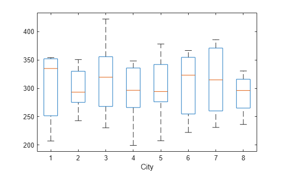

Box plot of the response grouped by city

The figure does not appear to show any systematic differences in the mean response among cities.

Plot Data Grouped by Different Category

To look for potential year-specific fixed effects, create a box plot of the response grouped by year.

figure
boxplot(y,year)
xlabel("Year")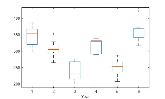

Box plot of the response grouped by year

Some evidence of systematic differences in the mean response between years seems to exist.

Format Response Data

Let $y_{i j}$ denote the response for city $j = 1, . . ., d$ , in year $i = 1, . . ., n$ . Similarly, $x_{i j}$ is the corresponding value of the predictor variable. In this example, $n = 6$ and $d = 8$ .

Consider fitting a year-specific fixed effects model with a constant slope and concurrent correlation among cities in the same year, $y_{i j} = α_{i} + β_{1} x_{i j} + ϵ_{i j}$ , where $ϵ_{i} = (ϵ_{i 1}, . . ., ϵ_{i d})^{'} \sim M V N (0, Σ)$ . The concurrent correlation accounts for any unmeasured, time-static factors that might impact growth similarly for some cities. For example, cities with close spatial proximity might be more likely to have similar economic growth.

To fit this model using mvregress, reshape the response data into an n-by-d matrix.

n = 6;
d = 8;
Y = reshape(y,n,d);

Format Design Matrices

Create a length-n cell array of d-by-K design matrices. For this model, there are $K = 7$ parameters ( $d = 6$ intercept terms and a slope).

Suppose the vector of parameters is arranged as $β = (\begin{array}{c} α_{1} \\ α_{2} \\ ⋮ \\ α_{6} \\ β_{1} \end{array})$ . In this case, the first design matrix for year 1 looks like $X {1} = (\begin{array}{ccccc} 1 & 0 & \dots & 0 & x_{11} \\ 1 & 0 & \dots & 0 & x_{12} \\ ⋮ & ⋮ & \dots & 0 & ⋮ \\ 1 & 0 & \dots & 0 & x_{18} \end{array})$ ,

and the second design matrix for year 2 looks like $X {2} = (\begin{array}{ccccc} 0 & 1 & 0 & \dots & 0 & x_{21} \\ 0 & 1 & 0 & \dots & 0 & x_{22} \\ ⋮ & ⋮ & ⋮ & \dots & 0 & ⋮ \\ 0 & 1 & 0 & \dots & 0 & x_{28} \end{array})$ . The design matrices for the remaining 4 years are similar.

K = 7;
N = n*d;
X = cell(n,1);
for i = 1:n
    x0 = zeros(d,K-1);
    x0(:,i) = 1;
    X{i} = [x0,x(i:n:N)];
end

Fit and Plot Model

Fit the model using ordinary least squares (OLS).

[b,sig,E,V] = mvregress(X,Y,Algorithm="cwls");
b

Plot the fitted model.

xx = linspace(min(x),max(x));
axx = repmat(b(1:K-1),1,length(xx));
bxx = repmat(b(K)*xx,n,1);
yhat =  axx + bxx;

figure
hPoints = gscatter(x,y,year);
hold on
hLines = plot(xx,yhat);
for i=1:n  
    set(hLines(i),"color",get(hPoints(i),"color"));
end
hold off
legend(["Year 1","Year 2","Year 3","Year 4", ...
    "Year 5","Year 6"],Location="bestoutside")

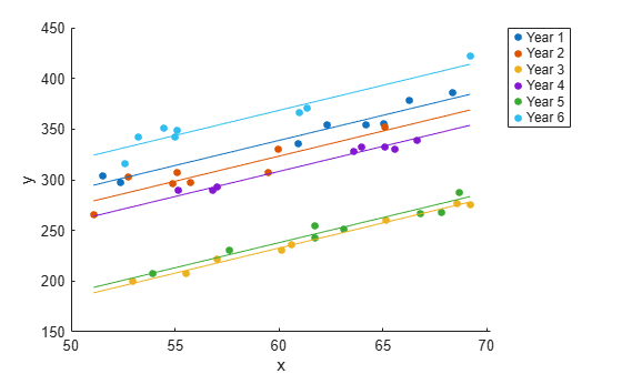
Plot of y versus x showing the data and fitted model for each year

The model with year-specific intercepts and common slope appears to fit the data quite well.

Visualize Residual Correlation

Plot the residuals, grouped by year.

figure
gscatter(year,E(:),city)
ylabel("Residuals")
legend(["City 1","City 2","City 3","City 4", ...
    "City 5","City 6","City 7","City 8"], ...
    Location="bestoutside")

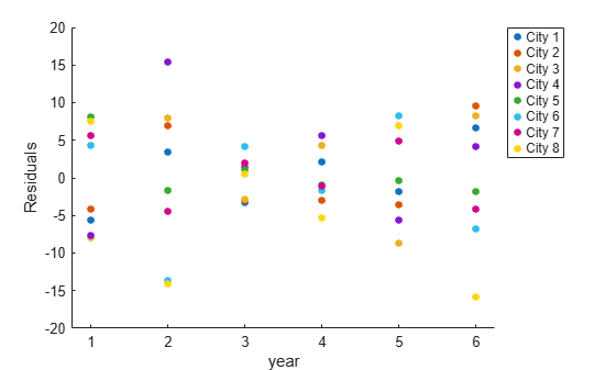
Scatter plot of residuals versus year for each city

The residual plot suggests concurrent correlation is present. For examples, cities 1, 2, 3, and 4 are consistently above or below average as a group in any given year. The same is true for the collection of cities 5, 6, 7, and 8. As seen in the exploratory plots, there are no systematic city-specific effects.

Compute Panel Corrected Standard Errors

Use the estimated error variance-covariance matrix to compute panel corrected standard errors for the regression coefficients.

XX = cell2mat(X);
S = kron(eye(n),sig);
Vpcse = inv(XX'*XX)*XX'*S*XX*inv(XX'*XX);
se = sqrt(diag(Vpcse))