Generate Constant Velocity Reference Path with Handling Limits

R2026b

This example shows how to use the Reference Path Generator block to generate a constant velocity reference for a path-following simulation and then apply curvature-based handling limits to adapt the velocity to path geometry. You configure block parameters for two cases and compare the results.

The example model includes a Simulation 3D Scene Configuration block that enables 3D visualization, allowing you to observe vehicle behavior in a realistic environment during simulation.

Open Model

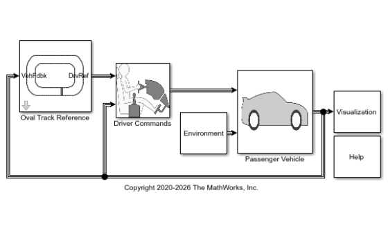
The vdynblksOvalTrack model simulates a 3 degree-of-freedom (DOF) vehicle driving around an oval track. The Oval Track Reference subsystem contains a Reference Path Generator block that reads waypoints and outputs reference pose, curvature, and velocity signals. A Linear Predictive Driver steers the vehicle along the path and tracks the velocity reference. A Powertrain and Driveline subsystem scales the driver command into tractive and braking torques. The vehicle is a Vehicle Body 3DOF block.

Open the model and enable 3D visualization. Turn off the low-beam lights so that tail lights do not illuminate in the 3D visualization.

mdl = "vdynblksOvalTrack";
open_system(mdl)
set_param(mdl, "ReturnWorkspaceOutputs", "on");
set_param(mdl + "/Visualization/3D Visualization", "engine3D", "Enabled - Ground Following");
set_param(mdl + "/Passenger Vehicle/Vehicle Body 3DOF Dual Track/Light Logic/Lowbeam", "Value", "false");
simulinkScreenshot(mdl)

Simulation 1: Constant Velocity Without Handling Limits

Configure the Reference Path Generator to output a constant velocity of 110 mph (49.17 m/s) along the entire path. Disable curvature-based constraints so the velocity reference remains constant regardless of path geometry.

blk = mdl + "/Oval Track Reference/Reference Path Generator";
set_param(blk, "velRefMode", "Constant");
set_param(blk, "velRef", "110");
set_param(blk, "velRefUnit", "mph");
set_param(blk, "velLim", "off");

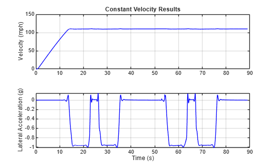
Run the simulation. Without handling limits, the vehicle attempts to maintain 110 mph through the curves, generating lateral forces that exceed the safe handling threshold.

simConstant = sim(mdl);

3D Visualization: Constant Velocity

The Simulation 3D Viewer shows the vehicle following the oval track at a constant 110 mph. Without handling limits, the vehicle maintains its target speed through curves, causing large lateral forces.

Constant Velocity Results

Extract the logged signals from the simulation output.

logsout1 = simConstant.logsout;
vel1 = logsout1.getElement("xdot_mph");
ay1 = logsout1.getElement("<ay>");
X1 = logsout1.getElement("<X>");
Y1 = logsout1.getElement("<Y>");
XRef1 = logsout1.getElement("XRef");
YRef1 = logsout1.getElement("YRef");

Plot longitudinal velocity in mph and lateral acceleration in g for the constant velocity simulation. Blue lines represent the constant velocity signals. The lateral acceleration exceeds safe handling limits as the vehicle negotiates the curves.

figure
subplot(2,1,1)
plot(vel1.Values.Time, vel1.Values.Data, "b-")
ylim([0 150])
ylabel("Velocity (mph)")
title("Constant Velocity Results")
grid on
subplot(2,1,2)
plot(ay1.Values.Time, ay1.Values.Data, "b-")
xlabel("Time (s)")
ylabel("Lateral Acceleration (g)")
grid on

Simulation 2: Constant Velocity with Handling Limits

Enable curvature-based velocity constraints. The Reference Path Generator block uses path curvature to compute the maximum safe speed at each point:

$$v_{\max }=\sqrt{a_{y,\max }\cdot R};$$

where $$R=1/|\kappa |$$ is the radius of curvature. Forward and backward passes enforce tractive and braking acceleration limits to produce smooth speed transitions when entering and exiting curves.

A safe lateral acceleration limit depends on the tire-road friction capacity, road conditions, and vehicle characteristics. Setting the limit below the peak friction capacity leaves margin for surface variations, transient maneuvers, and combined braking-cornering loads.

For this simulation, limit the lateral acceleration to 0.5 g. Set the constraint parameters:

• Lateral acceleration limit, ayMax: 0.5 g

• Braking deceleration limit, axMin: -0.8 g

• Tractive acceleration limit, axMax: 0.5 g

• Minimum velocity, velRefMin: 80 mph

• Maximum velocity, velRefMax: 180 mph

set_param(blk, "velLim", "on");
set_param(blk, "ayMax", "0.5");
set_param(blk, "axMin", "-0.8");
set_param(blk, "axMax", "0.5");
set_param(blk, "velRefMin", "80");
set_param(blk, "velRefMax", "180");

Run the simulation. With handling limits, the vehicle slows before entering curves and completes the full lap around the oval track.

simLimited = sim(mdl);

3D Visualization: Handling-Limited

With curvature-based handling limits enabled, the vehicle slows before entering curves and accelerates on straights. The Simulation 3D Viewer shows smooth cornering and tight path tracking as the vehicle completes the full lap.

Handling-Limited Results

Extract the logged signals from the simulation output.

logsout2 = simLimited.logsout;
vel2 = logsout2.getElement("xdot_mph");
ay2 = logsout2.getElement("<ay>");
X2 = logsout2.getElement("<X>");
Y2 = logsout2.getElement("<Y>");
XRef2 = logsout2.getElement("XRef");
YRef2 = logsout2.getElement("YRef");

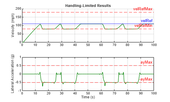
Plot longitudinal velocity in mph and lateral acceleration in g for the handling-limited simulation. The velocity reference (blue) is the constant 110 mph target set by the velRef parameter. The actual lateral acceleration briefly exceeds the ayMax limit because the handling limits constrain the velocity reference, not the vehicle dynamics directly. The vehicle has inertia and the driver model has a finite response, so actual lateral acceleration can overshoot during curve entry transients.

figure
subplot(2,1,1)
yline(110, "b-", "velRef")
hold on
plot(vel2.Values.Time, vel2.Values.Data, "-", Color=[0 0.5 0])
yline(80, "r--", "velRefMin")
yline(180, "r--", "velRefMax")
hold off
ylabel("Velocity (mph)")
title("Handling-Limited Results")
grid on
subplot(2,1,2)
plot(ay2.Values.Time, ay2.Values.Data, "-", Color=[0 0.5 0])
hold on
yline(0.5, "r--", "ayMax")
yline(-0.5, "r--", "-ayMax")
hold off
ylim([-1 1])
xlabel("Time (s)")
ylabel("Lateral Acceleration (g)")
grid on

Compare Results

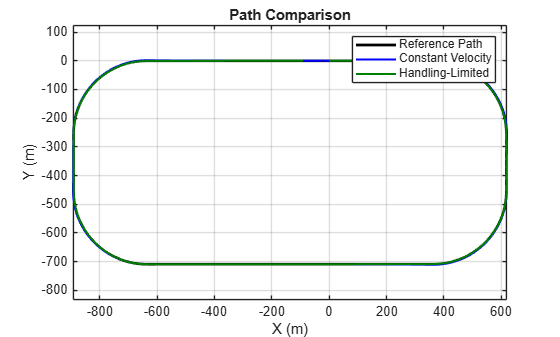
Plot the reference path alongside the actual vehicle paths from both simulations. Without handling limits, the vehicle exhibits noticeable tracking errors in curves. With handling limits, the vehicle tracks the reference path closely.

figure
plot(squeeze(XRef1.Values.Data), squeeze(YRef1.Values.Data), "k-", LineWidth=2)
hold on
plot(X1.Values.Data, Y1.Values.Data, "b-", LineWidth=1.5)
plot(X2.Values.Data, Y2.Values.Data, "-", Color=[0 0.5 0], LineWidth=1.5)
hold off
xlabel("X (m)")
ylabel("Y (m)")
title("Path Comparison")
legend("Reference Path", "Constant Velocity", "Handling-Limited")
axis equal
grid on

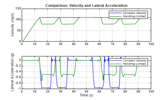
Overlay velocity and lateral acceleration from both simulations. The handling-limited velocity profile slows for curves, while the constant velocity case maintains speed and generates excessive lateral acceleration.

figure
subplot(2,1,1)
plot(vel1.Values.Time, vel1.Values.Data, "b-");
hold on; plot(vel2.Values.Time, vel2.Values.Data, "-", Color=[0 0.5 0]); hold off
ylim([0 150])
ylabel("Velocity (mph)")
title("Comparison: Velocity and Lateral Acceleration")
legend("Constant Velocity", "Handling-Limited")
grid on
subplot(2,1,2)
plot(ay1.Values.Time, ay1.Values.Data, "b-");
hold on; plot(ay2.Values.Time, ay2.Values.Data, "-", Color=[0 0.5 0]); hold off
xlabel("Time (s)")
ylabel("Lateral Acceleration (g)")
legend("Constant Velocity", "Handling-Limited")
grid on

This example shows two velocity reference configurations for the Reference Path Generator block:

• Constant velocity — A single target speed along the entire path. Simple to configure, but the vehicle might exceed handling limits in curves, causing tracking errors.

• Constant velocity with handling limits — The block enforces curvature-based constraints using lateral acceleration, braking, and tractive limits. The velocity reference adapts to path geometry, slowing in curves and accelerating on straights.

When the reference path includes tight curves or high speeds, use curvature-based handling limits. The limits keep the velocity reference in the kinematic envelope of the vehicle, improving path tracking and reducing the risk of instability.