Automating Communications Measurement
By Mike Woodward, MathWorks
Automating communications measurement involves more than merely creating a push-button interface to control instruments. An ideal automated system combines data analysis, instrument control, and reporting. For example, such a system might fit a model to measured data, compare model predictions to new measurement data, and summarize the results in a document. Most currently available automated systems are good at one of these tasks but not others—for example, a solution might offer excellent instrument control but poor data analysis abilities.
This article shows how you can automate the entire measurement process in MATLAB®. We will demonstrate the automation through two examples. The first shows the combination of instrument control and data analysis in a MATLAB GUI. The second shows automated data analysis and report writing, and demonstrates how to create a standalone executable that can be shared with end users without exposing the underlying code.
The code samples discussed in this article are available for download.
Combining Instrument Control and Data Analysis
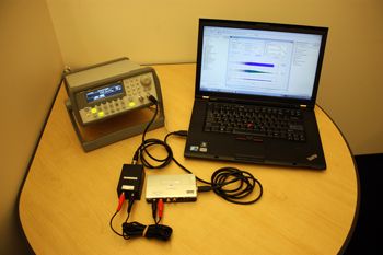
This example shows how you can combine measurement taking, data analysis, and visualization in one GUI-driven MATLAB application. Our goal is to model the response of an unknown circuit to a known input from an Agilent® 33220A arbitrary waveform generator. Our test setup consists of an unknown circuit, an external sound card to capture the output of the unknown circuit, the waveform generator, and, of course, MATLAB (Figure 1).
The first step is controlling test equipment from MATLAB using Instrument Control Toolbox™. The toolbox enables us to control equipment via a variety of interfaces, including USB, LXI, and GPIB. It also provides instrument-specific drivers for many instruments from Agilent, Tektronix, Rohde & Schwarz, and other vendors.
Controlling an instrument involves creating and opening a session using a protocol object, writing commands to the session, and reading the instrument’s response. We can connect to and control an Agilent 33220A arbitrary waveform generator via the VISA interface using the following code:
interfaceObj = visa('AGILENT', VISAaddress)
% Create a device object.
fgen = icdevice('agilent_33220a.mdd', interfaceObj)
% Connect device object to hardware.
connect(fgen)
% Set the voltage amplitude to 0.2 V
set(fgen, 'Amplitude', 0.2)
As you can see, the code is straightforward.
Next, using the GUIDE tools in MATLAB we build a GUI-based application for real-time instrument control, data analysis, and visualization. Via the GUI, the user controls the instrument settings and starts the measurement process (Figure 2).
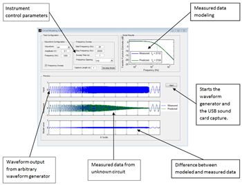
The application simultaneously receives data from the sound card and the waveform generator and displays it on the graphs. When the user clicks Develop Model, the underlying code analyzes the waveform data and the data from the unknown circuit, fitting a polynomial model to the data and displaying the fitting results as a function of signal frequency. When measurement-taking resumes after the model has been built, the application shows the difference between the measured and modeled data.
Data Analysis and GUI Building
Our second application continues the theme of GUI control, but this time, we want to automate data analysis and report writing. Our goal is to examine how certain measured Long Term Evolution (LTE) parameters vary over time. Amplifier and transmitter characteristics vary from device to device, but a trend over time may indicate a problem that we need to investigate. We want to display these variations and model changes.
Our source data is a file of measured LTE parameters such as maximum output power, EVM, receiver sensitivity, and spurious emissions for different devices acquired at different times.
GUI Building
We want to display variations in measured parameters over time and plot these variations as a histogram (to show the type of distribution and spread). We also want to obtain minimum, maximum, and mean values plus standard deviation. Our GUI will automate these tasks. Using the GUIDE tool, we build the interface (Figure 3).
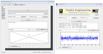
GUIDE uses a drag-and-drop approach, enabling you to build GUIs through a menu of GUI items, such as push buttons, text boxes, and graphs. We link GUI controls to the underlying MATLAB code via callback functions. For example, when the user clicks Update to update the graph, the application calls the following callback function. Note that the graphs include variation with time and histograms.
% --- Executes on button press in UpdateGraphs.
function UpdateGraphs_Callback(hObject, eventdata, handles)
axes(handles.axes1);
cla;
popup_sel_index = get(handles.popupmenu1, 'Value');
switch popup_sel_index
case 1
plot(handles.max_output);
case 2
hist(handles.max_output);
case 3
plot(handles.min_output);
case 4
hist(handles.min_output);
case 5
plot(handles.evm);
case 6
hist(handles.evm);
case 7
plot(handles.receive_sens);
case 8
hist(handles.receive_sens);
case 9
plot(handles.acs);
case 10
hist(handles.acs);
case 11
plot(handles.spurious_emi);
case 12
hist(handles.spurious_emi);
end
The underlying code could be any MATLAB code; for example, it could be code for controlling instruments, analyzing data, or drawing graphs.
Selecting buttons on the GUI activates the underlying code. For example, when the user clicks Browse, a dialog box opens to locate the data file. When the user selects Run analysis, the underlying code calculates statistics for each measured parameter and displays the results in a dialog box.
Automating Report Generation
Analyzing and writing reports on the variation of components and systems over time is a necessary but tedious task. MATLAB Report Generator™ automates much of the data analysis and report writing process.
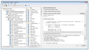
In the Report Generator tool, we define the structure of the report: an overview with summary results, and a section for each individual parameter. We write MATLAB code to calculate measurement statistics (minimum and maximum, mean, standard deviation), curve-fit data (to see if there is a variation over time), and generate graphs plotting parameter values against time and parameter histograms. We include this code in our Report Generator project and add the MATLAB output to our generated report (Figure 4).
At the press of a button we produce a Microsoft® Word® document containing all this information (Figure 5).
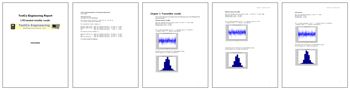
The report includes an overview with a summary of the results and a section for each parameter, including an analysis of variation over time (including an automated short assessment of whether the variation is significant), graphs, curve-fitting results, and parameter histogram. The Word document is editable, enabling interpretations of the data to be added to the basic report.
To further automate the process, we add report generation to the GUI. The Report Generator can be called from the MATLAB command line without going through the interface, so we can add a Generate Report button to the GUI and connect it to MATLAB code that generates the report.
Building Standalone Applications
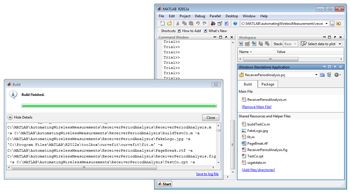
MATLAB Compiler™ lets you share an application while protecting the underlying source code. The compiler compiles applications into a standalone executable that users can run without having access to the source code or a MATLAB license.
The process is straightforward (Figure 6). The first step is to create a project file containing the MATLAB files and all other files needed by the application (for example, image files). This process is similar to building projects in other C compilers. The second step is to compile the project, which is simply a matter of pressing the Compile button. The last step is to distribute the standalone executable.
Standalone applications can include almost all MATLAB features, including data analysis, graphs, instrument control, statistical analysis, and signal processing.
We’ve built an application that can control instruments, analyze and display data, and produce written reports, and compiled the application for distribution as a standalone application. In short, we’ve automated the entire communications measurement process using MATLAB.
Published 2012 - 92060v00