Generate INT8 Code for Deep Learning Network on Raspberry Pi
Deep learning uses neural network architectures that contain many processing layers, including convolutional layers. Deep learning models typically work on large sets of labeled data. Performing inference on these models is computationally intensive, consuming significant amount of memory. Neural networks use memory to store input data, parameters (weights), and activations from each layer as the input propagates through the network. Deep Neural networks trained in MATLAB® use single-precision floating point data types. Even networks that are small in size require a considerable amount of memory and hardware to perform these floating-point arithmetic operations. These restrictions can inhibit deployment of deep learning models to devices that have low computational power and smaller memory resources. By using a lower precision to store the weights and activations, you can reduce the memory requirements of the network.
You can use Deep Learning Toolbox™ in tandem with the Deep Learning Toolbox Model Compression Library support package to reduce the memory footprint of a deep neural network by quantizing the weights, biases, and activations of convolution layers to 8-bit scaled integer data types. The quantization is performed by providing the calibration result file produced by the calibrate (Deep Learning Toolbox) function to the codegen command. Then, you can use MATLAB Coder™ to generate optimized code for the this network. The generated code takes advantage of ARM® processor SIMD by using the ARM Compute library. The generated code can be integrated into your project as source code, static or dynamic libraries, or executables that you can deploy to a variety of ARM CPU platforms such as Raspberry Pi®.
This example shows how to generate C++ code for a convolution neural network that uses the ARM Compute Library and performs inference computations in 8-bit integers.
This example is not supported for MATLAB Online™.
Third-Party Prerequisites
Raspberry Pi hardware
ARM Compute Library (on the target ARM hardware)
Environment variables for the compilers and libraries. See Prerequisites for Deep Learning with MATLAB Coder.
Example: Classify Images Using SqueezeNet
In this example, you use MATLAB Coder to generate optimized C++ code for a deep convolutional neural network and classify an image. The generated code performs inference computation using 8-bit integer data type for the convolution layer. The example uses the pretrained squeezenet (Deep Learning Toolbox) convolution neural network.
SqueezeNet has been trained on the ImageNet dataset containing images of 1000 object categories. The network has learned rich feature representations for a wide range of images. The network takes an image as input and outputs a label for the object in the image together with the probabilities for each of the object categories.
This example consists of four steps:
Modify the SqueezeNet neural network to classify a smaller subset of images containing five object categories using transfer learning.
Use the
calibratefunction to exercise the network with sample inputs and collect range information to produce a calibration result file.Generate optimized code for the network by using the codegen command and the calibration result file. The generated code runs on Raspberry Pi target via PIL execution.
Execute the generated PIL MEX on Raspberry Pi.
Transfer Learning Using SqueezeNet
To perform classification on a new set of images, you must fine-tune a pretrained SqueezeNet convolution neural network by using transfer learning. In transfer learning, you take a pretrained network and use it as a starting point to learn a new task. Fine-tuning a network by using transfer learning is usually much faster and easier than training a network with randomly initialized weights from scratch. You can quickly transfer learned features to a new task by using a smaller number of training images.
Load Training Data
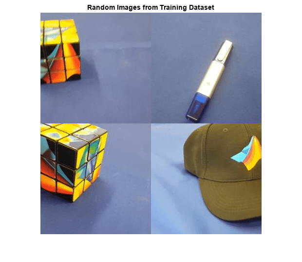
Unzip and load the new images as an image datastore. The imageDatastore function automatically labels the images based on folder names and stores the data as an ImageDatastore object. An image datastore enables you to store large image data, including data that does not fit in memory, and efficiently read batches of images during training of a convolution neural network.
unzip('MerchData.zip');
imds = imageDatastore('MerchData', ...
    'IncludeSubfolders',true, ...
    'LabelSource','foldernames');
[imdsTrain,imdsValidation] = splitEachLabel(imds,0.7,'randomized');

numTrainImages = numel(imdsTrain.Labels);
idx = randperm(numTrainImages,4);
img = imtile(imds, 'Frames', idx);

figure
imshow(img)
title('Random Images from Training Dataset');
Load Pretrained Network
Load the pretrained SqueezeNet network.
net=squeezenet;
The object net contains the DAGNetwork object. The first layer is the image input layer that accepts input images of size 227-by-227-by-3, where 3 is the number of color channels. Use the analyzeNetwork (Deep Learning Toolbox) function to display an interactive visualization of the network architecture, to detect errors and issues in the network, and to display detailed information about the network layers. The layer information includes the sizes of layer activations and learnable parameters, the total number of learnable parameters, and the sizes of state parameters of recurrent layers.
inputSize = net.Layers(1).InputSize;
analyzeNetwork(net);
Replace Final Layers
The convolutional layers of the network extract image features that the last learnable layer and the final classification layer use to classify the input image. These two layers, 'conv10' and 'ClassificationLayer_predictions' in SqueezeNet, contain information about how to combine the features that the network extracts into class probabilities, a loss value, and predicted labels.
To retrain a pretrained network to classify new images, replace these two layers with new layers adapted to the new data set. You can do this manually or use the helper function findLayersToReplace to find these layers automatically.
This is the findLayersToReplace helper function:
type findLayersToReplace.mfunction [learnableLayer,classLayer] = findLayersToReplace(lgraph)
% findLayersToReplace(lgraph) finds the single classification layer and the
% preceding learnable (fully connected or convolutional) layer of the layer
% graph lgraph.
% Copyright 2021 The MathWorks, Inc.
if ~isa(lgraph,'nnet.cnn.LayerGraph')
error('Argument must be a LayerGraph object.')
end
% Get source, destination, and layer names.
src = string(lgraph.Connections.Source);
dst = string(lgraph.Connections.Destination);
layerNames = string({lgraph.Layers.Name}');
% Find the classification layer. The layer graph must have a single
% classification layer.
isClassificationLayer = arrayfun(@(l) ...
(isa(l,'nnet.cnn.layer.ClassificationOutputLayer')|isa(l,'nnet.layer.ClassificationLayer')), ...
lgraph.Layers);
if sum(isClassificationLayer) ~= 1
error('Layer graph must have a single classification layer.')
end
classLayer = lgraph.Layers(isClassificationLayer);
% Traverse the layer graph in reverse starting from the classification
% layer. If the network branches, throw an error.
currentLayerIdx = find(isClassificationLayer);
while true
if numel(currentLayerIdx) ~= 1
error('Layer graph must have a single learnable layer preceding the classification layer.')
end
currentLayerType = class(lgraph.Layers(currentLayerIdx));
isLearnableLayer = ismember(currentLayerType, ...
['nnet.cnn.layer.FullyConnectedLayer','nnet.cnn.layer.Convolution2DLayer']);
if isLearnableLayer
learnableLayer = lgraph.Layers(currentLayerIdx);
return
end
currentDstIdx = find(layerNames(currentLayerIdx) == dst);
currentLayerIdx = find(src(currentDstIdx) == layerNames); %#ok<FNDSB>
end
end
To use this function to replace the final layers, run these commands:
lgraph = layerGraph(net);
[learnableLayer,classLayer] = findLayersToReplace(lgraph);
numClasses = numel(categories(imdsTrain.Labels));

newConvLayer =  convolution2dLayer([1, 1],numClasses,'WeightLearnRateFactor',...
10,'BiasLearnRateFactor',10,"Name",'new_conv');
lgraph = replaceLayer(lgraph,'conv10',newConvLayer);

newClassificatonLayer = classificationLayer('Name','new_classoutput');
lgraph = replaceLayer(lgraph,'ClassificationLayer_predictions',newClassificatonLayer);
Train Network
The network requires all input images to have the size 227-by-227-by-3, but each image in the image datastores has a different size. Use an augmented image datastore to automatically resize the training images. Specify these additional augmentation operations to be performed on the training images: randomly flip the training images about the vertical axis, and randomly translate them up to 30 pixels horizontally and vertically. Data augmentation helps prevent the network from over-fitting and memorizing the exact details of the training images.
pixelRange = [-30 30];
imageAugmenter = imageDataAugmenter( ...
    'RandXReflection',true, ...
    'RandXTranslation',pixelRange, ...
    'RandYTranslation',pixelRange);
augimdsTrain = augmentedImageDatastore(inputSize(1:2),imdsTrain, ...
    'DataAugmentation',imageAugmenter);
To automatically resize the validation images without performing further data augmentation, use an augmented image datastore without specifying any additional preprocessing operations.
augimdsValidation = augmentedImageDatastore(inputSize(1:2),imdsValidation);
Specify the training options. For transfer learning, keep the features from the early layers of the pretrained network (the transferred layer weights). To slow down learning in the transferred layers, set the initial learning rate to a small value. In the previous step, you increased the learning rate factors for the convolutional layer to speed up learning in the new final layers. This combination of learning rate settings results in fast learning only in the new layers and slower learning in the other layers. When performing transfer learning, you do not need to train for as many epochs. An epoch is a full training cycle on the entire training data set. Specify the mini-batch size to be 11 so that in each epoch you consider all of the data. During training, the software validates the network after every ValidationFrequency iterations.
options = trainingOptions('sgdm', ...
    'MiniBatchSize',11, ...
    'MaxEpochs',7, ...
    'InitialLearnRate',2e-4, ...
    'Shuffle','every-epoch', ...
    'ValidationData',augimdsValidation, ...
    'ValidationFrequency',3, ...
    'Verbose',false);
Train the network that consists of the transferred and new layers.
netTransfer = trainNetwork(augimdsTrain,lgraph,options);
classNames = netTransfer.Layers(end).Classes;
save('mySqueezenet.mat','netTransfer');
Generate Calibration Result File for the Network
Create a dlquantizer object and specify the network. Note that code generation does not support quantized deep neural networks produced by the quantize (Deep Learning Toolbox) function.
quantObj = dlquantizer(netTransfer, 'ExecutionEnvironment', 'CPU');
Use the calibrate function to exercise the network with sample inputs and collect range information. The calibrate function exercises the network and collects the dynamic ranges of the weights and biases in the convolution and fully connected layers of the network and the dynamic ranges of the activations in all layers of the network. The function returns a table. Each row of the table contains range information for a learnable parameter of the optimized network.
calResults = quantObj.calibrate(augimdsTrain);
save('squeezenetCalResults.mat','calResults');
save('squeezenetQuantObj.mat','quantObj');
Generate PIL MEX Function
In this example, you generate code for the entry-point function predict_int8. This function uses the coder.loadDeepLearningNetwork function to load a deep learning model and to construct and set up a CNN class. Then the entry-point function predicts the responses by using the predict (Deep Learning Toolbox) function.
type predict_int8.mfunction out = predict_int8(netFile, in)
persistent mynet;
if isempty(mynet)
mynet = coder.loadDeepLearningNetwork(netFile);
end
out = predict(mynet,in);
end
To generate a PIL MEX function, create a code configuration object for a static library and set the verification mode to 'PIL'. Set the target language to C++.
 cfg = coder.config('lib', 'ecoder', true);
 cfg.VerificationMode = 'PIL';
 cfg.TargetLang = 'C++';
Create a deep learning configuration object for the ARM Compute library. Specify the library version and arm architecture. For this example, suppose that the ARM Compute Library in the Raspberry Pi hardware is version 20.02.1.
 dlcfg = coder.DeepLearningConfig('arm-compute');
 dlcfg.ArmComputeVersion = '20.02.1';
 dlcfg.ArmArchitecture = 'armv7';
Set the properties of dlcfg to generate code for low precision/INT8 inference.
 dlcfg.CalibrationResultFile = 'squeezenetQuantObj.mat';
 dlcfg.DataType = 'int8';
6. Set the DeepLearningConfig property of cfg to dlcfg.
cfg.DeepLearningConfig = dlcfg;
7. Use the Raspberry Pi® Blockset function, raspi, to create a connection to the Raspberry Pi. In the following code, replace:
raspinamewith the name of your Raspberry Piusernamewith your user namepasswordwith your password
% r = raspi('raspiname','username','password'); 8. Create a coder.Hardware object for Raspberry Pi and attach it to the code generation configuration object.
% hw = coder.hardware('Raspberry Pi');
% cfg.Hardware = hw;
9. Generate a PIL MEX function by using the codegen command
% codegen -config cfg predict_int8 -args {coder.Constant('mySqueezenet.mat'), ones(227,227,3,'uint8')}Run Generated PIL MEX Function on Raspberry Pi
Input image is expected to be of same size as the input size of the network. Read the image that you want to classify and resize it to the input size of the network. This resizing slightly changes the aspect ratio of the image.
% testImage = imread("MerchDataTest.jpg");
% testImage = imresize(testImage,inputSize(1:2));
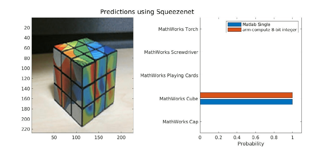
To compare the predictions of the Deep Learning Toolbox predict function and the generated PIL MEX function predict_int8_pil, call both these functions on the input image separately.
% predictScores(:,1) =  predict(netTransfer,testImage)';
% predictScores(:,2) = predict_int8_pil('mySqueezenet.mat',testImage)';
Display the predicted labels and their associated probabilities as a histogram.
% h = figure;
% h.Position(3) = 2*h.Position(3);
% ax1 = subplot(1,2,1);
% ax2 = subplot(1,2,2);
% image(ax1,testImage);
% barh(ax2,predictScores)
% xlabel(ax2,'Probability')
% yticklabels(ax2,classNames)
% ax2.XLim = [0 1.1];
% ax2.YAxisLocation = 'left';
% legend('Matlab Single','arm-compute 8-bit integer');
% sgtitle('Predictions using Squeezenet')
% saveas(gcf,'SqueeznetPredictionComparison.jpg');
% close(gcf);
imshow('SqueeznetPredictionComparison.jpg');
See Also
Apps
- Deep Network Quantizer (Deep Learning Toolbox)
Functions
dlquantizer(Deep Learning Toolbox) |dlquantizationOptions(Deep Learning Toolbox) |calibrate(Deep Learning Toolbox) |validate(Deep Learning Toolbox) |coder.loadDeepLearningNetwork|codegen