Convolutional Codes

Convolutional coding is a type of error-control coding distinguished by its use of memory, in contrast to block coders, which are memoryless. Although a convolutional coder processes a fixed number of input message symbols and generates a fixed number of output code symbols, its computations depend not only on the current input symbols but also on some of the previous input symbols.

Communications Toolbox™ provides convolutional coding capabilities as MATLAB^® functions and System objects, and Simulink^® blocks. The features support feedforward and feedback convolutional codes that can be described by a trellis structure or a set of generator polynomials and use the Viterbi algorithm to implement hard-decision and soft-decision decoding. The software also includes an a posteriori probability decoder, which can be used for soft output decoding of convolutional codes.

Use these features to generate various convolutional codes.

	Functions	System objects	Blocks
Convolutional	`convenc`, `vitdec`	`comm.APPDecoder`, `comm.ConvolutionalEncoder`, `comm.gpu.ConvolutionalEncoder`, `comm.ViterbiDecoder`	APP Decoder, Convolutional Encoder, Viterbi Decoder
Concatenated	—	`comm.TurboEncoder`, `comm.TurboDecoder`, `comm.gpu.TurboDecoder`,	Turbo Encoder, Turbo Decoder
Utilities	`distspec`, `getTurboIOIndices`, `iscatastrophic`, `istrellis`, `oct2dec`, `poly2trellis`	—	—

For background information about convolutional coding, see the works listed in Selected Bibliography for Convolutional Coding.

Convolutional Code Features

Block Parameters for Convolutional Coding

To process convolutional codes, use the Convolutional Encoder, Viterbi Decoder, and/or APP Decoder blocks in the Convolutional sublibrary. If a mask parameter is required in both the encoder and the decoder, use the same value in both blocks.

The blocks in the Convolutional sublibrary assume that you use one of two different representations of a convolutional encoder:

If you design your encoder using a diagram with shift registers and modulo-2 adders, you can compute the code generator polynomial matrix and subsequently use the poly2trellis function (in Communications Toolbox) to generate the corresponding trellis structure mask parameter automatically. For an example, see Design a Rate 2/3 Feedforward Encoder Using Simulink.
If you design your encoder using a trellis diagram, you can construct the trellis structure in MATLAB and use it as the mask parameter.

For more information about these representations, see Polynomial Description of a Convolutional Code and Trellis Description of a Convolutional Code.

Using the Polynomial Description in Blocks

To use the polynomial description with the Convolutional Encoder, Viterbi Decoder, or APP Decoder blocks, use the utility function poly2trellis from Communications Toolbox. This function accepts a polynomial description and converts it into a trellis description. For example, the following command computes the trellis description of an encoder whose constraint length is 5 and whose generator polynomials are 35 and 31:

trellis = poly2trellis(5,[35 31]);

To use this encoder with one of the convolutional-coding blocks, simply place a poly2trellis command such as

poly2trellis(5,[35 31]);

in the Trellis structure parameter field.

Polynomial Description of a Convolutional Code

A polynomial description of a convolutional encoder describes the connections among shift registers and modulo 2 adders. For example, the figure below depicts a feedforward convolutional encoder that has one input, two outputs, and two shift registers.

Feedforward convolutional encoder with one input, two outputs, and two shift registers.

A polynomial description of a convolutional encoder has either two or three components, depending on whether the encoder is a feedforward or feedback type:

Constraint lengths
Generator polynomials
Feedback connection polynomials (for feedback encoders only)

Constraint Lengths

The constraint lengths of the encoder form a vector whose length is the number of inputs in the encoder diagram. The elements of this vector indicate the number of bits stored in each shift register, including the current input bits.

In the figure above, the constraint length is three. It is a scalar because the encoder has one input stream, and its value is one plus the number of shift registers for that input.

Generator Polynomials

If the encoder diagram has k inputs and n outputs, the code generator matrix is a k-by-n matrix. The element in the ith row and jth column indicates how the ith input contributes to the jth output.

For systematic bits of a systematic feedback encoder, match the entry in the code generator matrix with the corresponding element of the feedback connection vector. See Feedback Connection Polynomials below for details.

In other situations, you can determine the (i,j) entry in the matrix as follows:

Build a binary number representation by placing a 1 in each spot where a connection line from the shift register feeds into the adder, and a 0 elsewhere. The leftmost spot in the binary number represents the current input, while the rightmost spot represents the oldest input that still remains in the shift register.
Convert this binary representation into an octal representation by considering consecutive triplets of bits, starting from the rightmost bit. The rightmost bit in each triplet is the least significant. If the number of bits is not a multiple of three, place zero bits at the left end as necessary. (For example, interpret 1101010 as 001 101 010 and convert it to 152.)

For example, the binary numbers corresponding to the upper and lower adders in the figure above are 110 and 111, respectively. These binary numbers are equivalent to the octal numbers 6 and 7, respectively, so the generator polynomial matrix is [6 7].

Note

You can perform the binary-to-octal conversion in MATLAB by using code like str2num(dec2base(bin2dec('110'),8)).

For a table of some good convolutional code generators, refer to [2] in the section Selected Bibliography for Block Coding, especially that book's appendices.

Feedback Connection Polynomials

If you are representing a feedback encoder, you need a vector of feedback connection polynomials. The length of this vector is the number of inputs in the encoder diagram. The elements of this vector indicate the feedback connection for each input, using an octal format. First build a binary number representation as in step 1 above. Then convert the binary representation into an octal representation as in step 2 above.

If the encoder has a feedback configuration and is also systematic, the code generator and feedback connection parameters corresponding to the systematic bits must have the same values.

Use Trellis Structure for Rate 1/2 Feedback Convolutional Encoder

Open Live Script

Create a trellis structure to represent the rate 1/2 systematic convolutional encoder with feedback shown in this diagram.

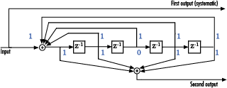
This encoder has 5 for its constraint length, [37 33] as its generator polynomial matrix, and 37 for its feedback connection polynomial.

The first generator polynomial is octal 37. The second generator polynomial is octal 33. The feedback polynomial is octal 37. The first generator polynomial matches the feedback connection polynomial because the first output corresponds to the systematic bits.

The binary vector [1 1 1 1 1] represents octal 37 and corresponds to the upper row of binary digits in the diagram. The binary vector [1 1 0 1 1] represents octal 33 and corresponds to the lower row of binary digits in the diagram. These binary digits indicate connections from the outputs of the registers to the two adders in the diagram. The initial 1 corresponds to the input bit.

Convert the polynomial to a trellis structure by using the poly2trellis function. When used with a feedback polynomial, poly2trellis makes a feedback connection to the input of the trellis.

trellis = poly2trellis(5,[37 33],37)

trellis = struct with fields:
     numInputSymbols: 2
    numOutputSymbols: 4
           numStates: 16
          nextStates: [16×2 double]
             outputs: [16×2 double]

Generate random binary data. Convolutionally encode the data by using the specified trellis structure. Decode the coded data by using the Viterbi algorithm with the specified trellis structure, 34 for its traceback depth, truncated operation mode, and hard decisions.

data = randi([0 1],70,1);
codedData = convenc(data,trellis);
tbdepth = 34; % Traceback depth for Viterbi decoder
decodedData = vitdec(codedData,trellis,tbdepth,'trunc','hard');

Verify the decoded data has zero bit errors.

biterr(data,decodedData)

ans = 
0

Using the Polynomial Description in MATLAB

To use the polynomial description with the convenc and vitdec functions, first convert the polynomial into a trellis description by using the poly2trellis function. For example, the command below computes the trellis description of the encoder pictured in the section Polynomial Description of a Convolutional Code.

trellis = poly2trellis(3,[6 7]);

The MATLAB structure trellis is a suitable input argument for convenc and vitdec.

Trellis Description of a Convolutional Code

A trellis description of a convolutional encoder shows how each possible input to the encoder influences both the output and the state transitions of the encoder. This section describes trellises, and how to represent trellises in MATLAB, and gives an example of a MATLAB trellis.

The figure below depicts a trellis for the convolutional encoder from the previous section. The encoder has four states (numbered in binary from 00 to 11), a one-bit input, and a two-bit output. (The ratio of input bits to output bits makes this encoder a rate-1/2 encoder.) Each solid arrow shows how the encoder changes its state if the current input is zero, and each dashed arrow shows how the encoder changes its state if the current input is one. The octal numbers above each arrow indicate the current output of the encoder.

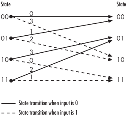
Trellis state diagram for the convolutional encoder from the previous section.

As an example of interpreting this trellis diagram, if the encoder is in the 10 state and receives an input of zero, it outputs the code symbol 3 and changes to the 01 state. If it is in the 10 state and receives an input of one, it outputs the code symbol 0 and changes to the 11 state.

Note that any polynomial description of a convolutional encoder is equivalent to some trellis description, although some trellises have no corresponding polynomial descriptions.

Specifying a Trellis in MATLAB

To specify a trellis in MATLAB, use a specific form of a MATLAB structure called a trellis structure. A trellis structure must have five fields, as in the table below.

Fields of a Trellis Structure for a Rate k/n Code

Field in Trellis Structure	Dimensions	Meaning
`numInputSymbols`	Scalar	Number of input symbols to the encoder: 2^k
`numOutputsymbols`	Scalar	Number of output symbols from the encoder: 2ⁿ
`numStates`	Scalar	Number of states in the encoder
`nextStates`	`numStates`-by-2^k matrix	Next states for all combinations of current state and current input
`outputs`	`numStates`-by-2^k matrix	Outputs (in octal) for all combinations of current state and current input

Note

While your trellis structure can have any name, its fields must have the exact names as in the table. Field names are case sensitive.

In the nextStates matrix, each entry is an integer between 0 and numStates-1. The element in the ith row and jth column denotes the next state when the starting state is i-1 and the input bits have decimal representation j-1. To convert the input bits to a decimal value, use the first input bit as the most significant bit (MSB). For example, the second column of the nextStates matrix stores the next states when the current set of input values is {0,...,0,1}. To learn how to assign numbers to states, see the reference page for istrellis.

In the outputs matrix, the element in the ith row and jth column denotes the encoder's output when the starting state is i-1 and the input bits have decimal representation j-1. To convert to decimal value, use the first output bit as the MSB.

How to Create a MATLAB Trellis Structure

Once you know what information you want to put into each field, you can create a trellis structure in any of these ways:

Define each of the five fields individually, using structurename.fieldname notation. For example, set the first field of a structure called s using the command below. Use additional commands to define the other fields.
```
s.numInputSymbols = 2;
```
The reference page for the istrellis function illustrates this approach.

Collect all field names and their values in a single struct command. For example:

s = struct('numInputSymbols',2,'numOutputSymbols',2,...
   'numStates',2,'nextStates',[0 1;0 1],'outputs',[0 0;1 1]);

Start with a polynomial description of the encoder and use the poly2trellis function to convert it to a valid trellis structure. For more information , see Polynomial Description of a Convolutional Code.

To check whether your structure is a valid trellis structure, use the istrellis function.

Example: A MATLAB Trellis Structure

Consider the trellis shown below.

Trellis state diagram.

To build a trellis structure that describes it, use the command below.

trellis = struct('numInputSymbols',2,'numOutputSymbols',4,...
'numStates',4,'nextStates',[0 2;0 2;1 3;1 3],...
'outputs',[0 3;1 2;3 0;2 1]);

The number of input symbols is 2 because the trellis diagram has two types of input path: the solid arrow and the dashed arrow. The number of output symbols is 4 because the numbers above the arrows can be either 0, 1, 2, or 3. The number of states is 4 because there are four bullets on the left side of the trellis diagram (equivalently, four on the right side). To compute the matrix of next states, create a matrix whose rows correspond to the four current states on the left side of the trellis, whose columns correspond to the inputs of 0 and 1, and whose elements give the next states at the end of the arrows on the right side of the trellis. To compute the matrix of outputs, create a matrix whose rows and columns are as in the next states matrix, but whose elements give the octal outputs shown above the arrows in the trellis.

Create and Decode Convolutional Codes

The functions for encoding and decoding convolutional codes are convenc and vitdec. This section discusses using these functions to create and decode convolutional codes.

Encoding

A simple way to use convenc to create a convolutional code is shown in the commands below.

% Define a trellis.
t = poly2trellis([4 3],[4 5 17;7 4 2]);
% Encode a vector of ones.
x = ones(100,1);
code = convenc(x,t);

The first command converts a polynomial description of a feedforward convolutional encoder to the corresponding trellis description. The second command encodes 100 bits, or 50 two-bit symbols. Because the code rate in this example is 2/3, the output vector code contains 150 bits (that is, 100 input bits times 3/2).

To check whether your trellis corresponds to a catastrophic convolutional code, use the iscatastrophic function.

Hard-Decision Decoding

To decode using hard decisions, use the vitdec function with the flag 'hard' and with binary input data. Because the output of convenc is binary, hard-decision decoding can use the output of convenc directly, without additional processing. This example extends the previous example and implements hard-decision decoding.

Define a trellis.

t = poly2trellis([4 3],[4 5 17;7 4 2]);
Encode a vector of ones.

code = convenc(ones(100,1),t);
Set the traceback length for decoding and decode using vitdec.

tb = 2;
decoded = vitdec(code,t,tb,'trunc','hard');
Verify that the decoded data is a vector of 100 ones.

isequal(decoded,ones(100,1))

ans = logical
   1

Soft-Decision Decoding

To decode using soft decisions, use the vitdec function with the flag 'soft'. Specify the number, nsdec, of soft-decision bits and use input data consisting of integers between 0 and 2^nsdec-1.

An input of 0 represents the most confident 0, while an input of 2^nsdec-1 represents the most confident 1. Other values represent less confident decisions. For example, the table below lists interpretations of values for 3-bit soft decisions.

Input Values for 3-bit Soft Decisions

Input Value	Interpretation
0	Most confident 0
1	Second most confident 0
2	Third most confident 0
3	Least confident 0
4	Least confident 1
5	Third most confident 1
6	Second most confident 1
7	Most confident 1

Implement Soft-Decision Decoding Using MATLAB

The script below illustrates decoding with 3-bit soft decisions. First it creates a convolutional code with convenc and adds white Gaussian noise to the code with awgn. Then, to prepare for soft-decision decoding, the example uses quantiz to map the noisy data values to appropriate decision-value integers between 0 and 7. The second argument in quantiz is a partition vector that determines which data values map to 0, 1, 2, etc. The partition is chosen so that values near 0 map to 0, and values near 1 map to 7. (You can refine the partition to obtain better decoding performance if your application requires it.) Finally, the example decodes the code and computes the bit error rate. When comparing the decoded data with the original message, the example must take the decoding delay into account. The continuous operation mode of vitdec causes a delay equal to the traceback length, so msg(1) corresponds to decoded(tblen+1) rather than to decoded(1).

s = RandStream.create('mt19937ar', 'seed',94384);
prevStream = RandStream.setGlobalStream(s);
msg = randi([0 1],4000,1); % Random data
t = poly2trellis(7,[171 133]); % Define trellis.
% Create a ConvolutionalEncoder System object
hConvEnc = comm.ConvolutionalEncoder(t);
% Create an AWGNChannel System object.
hChan = comm.AWGNChannel('NoiseMethod', 'Signal to noise ratio (SNR)',...
  'SNR', 6);
% Create a ViterbiDecoder System object
hVitDec = comm.ViterbiDecoder(t, 'InputFormat', 'Soft', ...
    'SoftInputWordLength', 3, 'TracebackDepth', 48, ...
    'TerminationMethod', 'Continuous');
% Create a ErrorRate Calculator System object. Account for the receive
% delay caused by the traceback length of the viterbi decoder.
hErrorCalc = comm.ErrorRate('ReceiveDelay', 48);
ber = zeros(3,1); % Store BER values
code = step(hConvEnc,msg); % Encode the data.
hChan.SignalPower = (code'*code)/length(code);
ncode = step(hChan,code); % Add noise.

% Quantize to prepare for soft-decision decoding.
qcode = quantiz(ncode,[0.001,.1,.3,.5,.7,.9,.999]);

tblen = 48; delay = tblen; % Traceback length
decoded = step(hVitDec,qcode); % Decode.

% Compute bit error rate.
ber = step(hErrorCalc, msg, decoded);
ratio = ber(1)
number = ber(2)
RandStream.setGlobalStream(prevStream);

The output is below.

number =

     5


ratio =

    0.0013

Implement Soft-Decision Decoding Using Simulink

This example creates a rate 1/2 convolutional code using the model described in Overview of the Simulation. It uses a quantizer and the Viterbi Decoder block to perform soft-decision decoding.

Defining the Convolutional Code

The feedforward convolutional encoder in this example is depicted below.

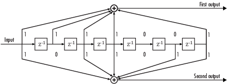
Feedforward convolutional encoder with one input, two outputs and six registers.

The encoder's constraint length is a scalar since the encoder has one input. The value of the constraint length is the number of bits stored in the shift register, including the current input. There are six memory registers, and the current input is one bit. Thus the constraint length of the code is 7.

The code generator is a 1-by-2 matrix of octal numbers because the encoder has one input and two outputs. The first element in the matrix indicates which input values contribute to the first output, and the second element in the matrix indicates which input values contribute to the second output.

For example, the first output in the encoder diagram is the modulo-2 sum of the rightmost and the four leftmost elements in the diagram's array of input values. The seven-digit binary number 1111001 captures this information, and is equivalent to the octal number 171. The octal number 171 thus becomes the first entry of the code generator matrix. Here, each triplet of bits uses the leftmost bit as the most significant bit. The second output corresponds to the binary number 1011011, which is equivalent to the octal number 133. The code generator is therefore [171 133].

The Trellis structure parameter in the Convolutional Encoder block tells the block which code to use when processing data. In this case, the poly2trellis function, in Communications Toolbox, converts the constraint length and the pair of octal numbers into a valid trellis structure.

While the message data entering the Convolutional Encoder block is a scalar bit stream, the encoded data leaving the block is a stream of binary vectors of length 2.

Mapping the Received Data

The received data, that is, the output of the AWGN Channel block, consists of complex numbers that are close to -1 and 1. In order to reconstruct the original binary message, the receiver part of the model must decode the convolutional code. The Viterbi Decoder block in this model expects its input data to be integers between 0 and 7. The demodulator, a custom subsystem in this model, transforms the received data into a format that the Viterbi Decoder block can interpret properly. More specifically, the demodulator subsystem

Converts the received data signal to a real signal by removing its imaginary part. It is reasonable to assume that the imaginary part of the received data does not contain essential information, because the imaginary part of the transmitted data is zero (ignoring small roundoff errors) and because the channel noise is not very powerful.
Normalizes the received data by dividing by the standard deviation of the noise estimate and then multiplying by -1.
Quantizes the normalized data using three bits.

The combination of this mapping and the Viterbi Decoder block's decision mapping reverses the BPSK modulation that the BPSK Modulator Baseband block performs on the transmitting side of this model. To examine the demodulator subsystem in more detail, double-click the icon labeled Soft-Output BPSK Demodulator.

Decoding the Convolutional Code

After the received data is properly mapped to length-2 vectors of 3-bit decision values, the Viterbi Decoder block decodes it. The block uses a soft-decision algorithm with 2³ different input values because the Decision type parameter is Soft Decision and the Number of soft decision bits parameter is 3.

Soft-Decision Interpretation of Data

When the Decision type parameter is set to Soft Decision, the Viterbi Decoder block requires input values between 0 and 2^b-1, where b is the Number of soft decision bits parameter. The block interprets 0 as the most confident decision that the codeword bit is a 0 and interprets 2^b-1 as the most confident decision that the codeword bit is a 1. The values in between these extremes represent less confident decisions. The following table lists the interpretations of the eight possible input values for this example.

Decision Value	Interpretation
0	Most confident 0
1	Second most confident 0
2	Third most confident 0
3	Least confident 0
4	Least confident 1
5	Third most confident 1
6	Second most confident 1
7	Most confident 1

Traceback and Decoding Delay

The traceback depth influences the decoding delay. The decoding delay is the number of zero symbols that precede the first decoded symbol in the output.

For the continuous operating mode, the decoding delay is equal to the number of traceback depth symbols.
For the truncated or terminated operating mode, the decoding delay is zero. In this case, the traceback depth must be less than or equal to the number of symbols in each input.

Traceback Depth Estimate

As a general estimate, a typical traceback depth value is approximately two to three times (ConstraintLength – 1) / (1 – coderate). The constraint length of the code, ConstraintLength, is equal to (log2(trellis.numStates) + 1). The coderate is equal to (K / N) × (length(PuncturePattern) / sum(PuncturePattern).

K is the number of input symbols, N is the number of output symbols, and PuncturePattern is the puncture pattern vector.

For example, applying this general estimate, results in these approximate traceback depths.

A rate 1/2 code has a traceback depth of 5 × (ConstraintLength – 1).
A rate 2/3 code has a traceback depth of 7.5 × (ConstraintLength – 1).
A rate 3/4 code has a traceback depth of 10 × (ConstraintLength – 1).
A rate 5/6 code has a traceback depth of 15 × (ConstraintLength – 1).

The Traceback depth parameter in the Viterbi Decoder block represents the length of the decoding delay. Some hardware implementations offer options of 48 and 96. This example chooses 48 because that is closer to the estimated target for a rate ½ code with a constraint length of 7.

Delay in Received Data

The Receive delay parameter of the Error Rate Calculation block is nonzero because a given message bit and its corresponding recovered bit are separated in time by a nonzero amount of simulation time. The Receive delay parameter tells the block which elements of its input signals to compare when checking for errors.

In this case, the Receive delay value is equal to the Traceback depth value (48).

Comparing Simulation Results with Theoretical Results

This section describes how to compare the bit error rate in this simulation with the bit error rate that would theoretically result from unquantized decoding. The process includes these steps

Computing Theoretical Bounds for the Bit Error Rate
To calculate theoretical bounds for the bit error rate P_b of the convolutional code in this model, you can use this estimate based on unquantized-decision decoding:
$P_{b} < \sum_{d = f}^{\infty} c_{d} P_{d}$
In this estimate, c_d is the sum of bit errors for error events of distance d, and f is the free distance of the code. The quantity P_d is the pairwise error probability, given by
$P_{d} = \frac{1}{2} erfc (\sqrt{d R \frac{E_{b}}{N_{0}}})$
where R is the code rate of 1/2, and erfc is the MATLAB complementary error function, defined by
$erfc (x) = \frac{2}{\sqrt{π}} \int_{x}^{\infty} e^{- t^{2}} d t$
Values for the coefficients c_d and the free distance f are in published articles such as "Convolutional Codes with Optimum Distance Spectrum" [3]. The free distance for this code is f = 10.
The following commands calculate the values of P_b for E_b/N₀ values in the range from 1 to 4, in increments of 0.5:
```
EbNoVec = [1:0.5:4.0];
R = 1/2;
% Errs is the vector of sums of bit errors for
% error events at distance d, for d from 10 to 29.
Errs = [36 0 211 0 1404 0 11633 0 77433 0 502690 0,...
        3322763 0 21292910 0 134365911 0 843425871 0]; 
% P is the matrix of pairwise error probilities, for
% Eb/No values in EbNoVec and d from 10 to 29.
P = zeros(20,7); % Initialize.
for d = 10:29
   P(d-9,:) = (1/2)*erfc(sqrt(d*R*10.^(EbNoVec/10)));
end
% Bounds is the vector of upper bounds for the bit error
% rate, for Eb/No values in EbNoVec.
Bounds = Errs*P;
```
Simulating Multiple Times to Collect Bit Error Rates
You can efficiently vary the simulation parameters by using the sim (Simulink) function to run the simulation from the MATLAB command line. For example, the following code calculates the bit error rate at bit energy-to-noise ratios ranging from 1 dB to 4 dB, in increments of 0.5 dB. It collects all bit error rates from these simulations in the matrix BERVec. It also plots the bit error rates in a figure window along with the theoretical bounds computed in the preceding code fragment.
This example simulates a rate 1/2 convolutional code using the model described in Overview of the Simulation. In the code sample below, the model name doc_softdecision represents the model described in Overview of the Simulation.
```
% Plot theoretical bounds and set up figure.
figure;
semilogy(EbNoVec,Bounds,'bo',1,NaN,'r*');
xlabel('Eb/No (dB)'); ylabel('Bit Error Rate');
title('Bit Error Rate (BER)');
l = legend('Theoretical bound on BER','Actual BER');
l.AutoUpdate = 'off';
axis([1 4 1e-5 1]);
hold on;

BERVec = [];
% Make the noise level variable.
set_param('doc_softdecision/AWGN Channel',...
    'EsNodB','EbNodB+10*log10(1/2)');
% Simulate multiple times.
for n = 1:length(EbNoVec)
    EbNodB = EbNoVec(n);
    sim('doc_softdecision',5000000);
    BERVec(n,:) = BER_Data;
    semilogy(EbNoVec(n),BERVec(n,1),'r*'); % Plot point.
    drawnow;
end
hold off;
```
Note
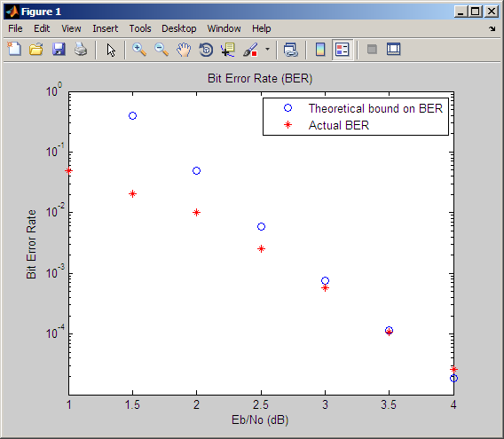
The estimate for P_b assumes that the decoder uses unquantized data, that is, an infinitely fine quantization. By contrast, the simulation in this example uses 8-level (3-bit) quantization. Because of this quantization, the simulated bit error rate is not quite as low as the bound when the signal-to-noise ratio is high.
The plot of bit error rate against signal-to-noise ratio follows. The locations of your actual BER points might vary because the simulation involves random numbers.

Design a Rate-2/3 Feedforward Encoder Using MATLAB

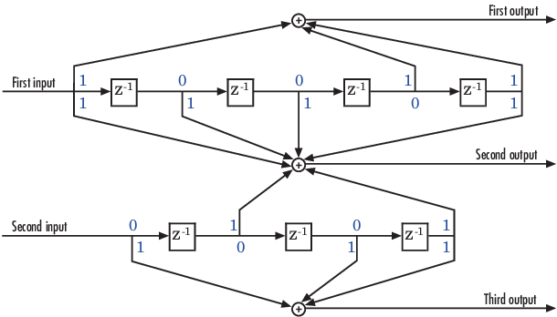
The example below uses the rate 2/3 feedforward encoder depicted in this schematic. The accompanying description explains how to determine the trellis structure parameter from a schematic of the encoder and then how to perform coding using this encoder.

$A block diagram of a rate 2/3 convolutional encoder with two inputs (labeled 'First Input' and 'Second Input' on the left side) and three outputs (labeled 'First Input', 'Second Output' and 'Third Output' on the right side). The first input passes through four delay elements labeled z^{-1}, with binary coefficients (1, 0, 1) along the branches. The second input passes through three delay elements labeled z^{-1}, also with binary coefficients (0, 1, 0, 1). The outputs are formed by summing selected branches: the first output combines paths from the first input, the second output combines paths from both inputs, and the third output combines paths from the second input. Each summation node is represented by a circle with a plus sign inside.$

Determining Coding Parameters

The convenc and vitdec functions can implement this code if their parameters have the appropriate values.

The encoder's constraint length is a vector of length 2 because the encoder has two inputs. The elements of this vector indicate the number of bits stored in each shift register, including the current input bits. Counting memory spaces in each shift register in the diagram and adding one for the current inputs leads to a constraint length of [5 4].

To determine the code generator parameter as a 2-by-3 matrix of octal numbers, use the element in the ith row and jth column to indicate how the ith input contributes to the jth output. For example, to compute the element in the second row and third column, the leftmost and two rightmost elements in the second shift register of the diagram feed into the sum that forms the third output. Capture this information as the binary number 1011, which is equivalent to the octal number 13. The full value of the code generator matrix is [23 35 0; 0 5 13].

To use the constraint length and code generator parameters in the convenc and vitdec functions, use the poly2trellis function to convert those parameters into a trellis structure. The command to do this is below.

trel = poly2trellis([5 4],[23 35 0;0 5 13]); % Define trellis.

Using the Encoder

Below is a script that uses this encoder.

len = 1000;

msg = randi([0 1],2*len,1); % Random binary message of 2-bit symbols
trel = poly2trellis([5 4],[23 35 0;0 5 13]); % Trellis
% Create a ConvolutionalEncoder System object
hConvEnc = comm.ConvolutionalEncoder(trel);
% Create a ViterbiDecoder System object
hVitDec = comm.ViterbiDecoder(trel, 'InputFormat', 'hard', ...
    'TracebackDepth', 34, 'TerminationMethod', 'Continuous');
% Create a ErrorRate Calculator System object. Since each symbol represents
% two bits, the receive delay for this object is twice the traceback length
% of the viterbi decoder.
hErrorCalc = comm.ErrorRate('ReceiveDelay', 68);
ber = zeros(3,1); % Store BER values
code = step(hConvEnc,msg); % Encode the message.
ncode = rem(code + randerr(3*len,1,[0 1;.96 .04]),2); % Add noise.
decoded = step(hVitDec, ncode); % Decode.
ber = step(hErrorCalc, msg, decoded);

convenc accepts a vector containing 2-bit symbols and produces a vector containing 3-bit symbols, while vitdec does the opposite. Also notice that biterr ignores the first 68 elements of decoded. That is, the decoding delay is 68, which is the number of bits per symbol (2) of the recovered message times the traceback depth value (34) in the vitdec function. The first 68 elements of decoded are 0s, while subsequent elements represent the decoded messages.

Design a Rate 2/3 Feedforward Encoder Using Simulink

This example uses the rate 2/3 feedforward convolutional encoder depicted in the following figure. The description explains how to determine the coding blocks' parameters from a schematic of a rate 2/3 feedforward encoder. This example also illustrates the use of the Error Rate Calculation block with a receive delay.

Rate 2/3 feedforward convolutional encoder with four registers.

How to Determine Coding Parameters

The Convolutional Encoder and Viterbi Decoder blocks can implement this code if their parameters have the appropriate values.

The encoder's constraint length is a vector of length 2 since the encoder has two inputs. The elements of this vector indicate the number of bits stored in each shift register, including the current input bits. Counting memory spaces in each shift register in the diagram and adding one for the current inputs leads to a constraint length of [5 4].

To determine the code generator parameter as a 2-by-3 matrix of octal numbers, use the element in the ith row and jth column to indicate how the ith input contributes to the jth output. For example, to compute the element in the second row and third column, notice that the leftmost and two rightmost elements in the second shift register of the diagram feed into the sum that forms the third output. Capture this information as the binary number 1011, which is equivalent to the octal number 13. The full value of the code generator matrix is [27 33 0; 0 5 13].

To use the constraint length and code generator parameters in the Convolutional Encoder and Viterbi Decoder blocks, use the poly2trellis function to convert those parameters into a trellis structure.

How to Simulate the Encoder

The following model simulates this encoder.

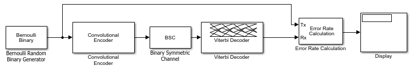
Simulink model showing convolutional encoding and Viterbi decoding impaired in a binary symmetric channel.

To build the model, gather and configure these blocks:

Bernoulli Binary Generator, with these updates to parameter settings:
- Set Probability of a zero to .5.
- Set Initial seed to any positive integer scalar, preferably the output of the randn function.
- Set Sample time to .5.
- Check the Frame-based outputs check box.
- Set Samples per frame to 2.
Convolutional Encoder, with these updates to parameter settings:
- Set Trellis structure to poly2trellis([5 4],[23 35 0; 0 5 13]).
Binary Symmetric Channel, in the Channels library
- Set Error probability to 0.02.
- Set Initial seed to any positive integer scalar, preferably the output of the randn function.
- Clear the Output error vector check box.
Viterbi Decoder, with these updates to parameter settings:
- Set Trellis structure to poly2trellis([5 4],[23 35 0; 0 5 13]).
- Set Decision type to Hard decision.
Error Rate Calculation, with these updates to parameter settings:
- Set Receive delay to 68.
- Set Output data to Port.
- Check the Stop simulation check box.
- Set Target number of errors to 100.
Display (Simulink)
- Drag the bottom edge of the icon to make the display big enough for three entries.

Connect the blocks as shown in the preceding figure. On the Simulation tab, in the Simulate section, set Stop time to inf. The Simulate section appears on multiple tabs.

Notes on the Model

You can display the matrix size of signals in your model. On the Debug tab, expand Information Overlays. In the Signals section, select Signal Dimensions.

The encoder accepts a 2-by-1 column vector and produces a 3-by-1 column vector, while the decoder does the opposite. The Samples per frame parameter in the Bernoulli Binary Generator block is 2 because the block must generate a message word of length 2.

The Receive delay parameter in the Error Rate Calculation block is 68, which is the vector length (2) of the recovered message times the Traceback depth value (34) in the Viterbi Decoder block. If you examine the transmitted and received signals as matrices in the MATLAB workspace, you see that the first 34 rows of the recovered message consist of zeros, while subsequent rows are the decoded messages. Thus the delay in the received signal is 34 vectors of length 2, or 68 samples.

Running the model produces display output consisting of three numbers: the error rate, the total number of errors, and the total number of comparisons that the Error Rate Calculation block makes during the simulation. (The first two numbers vary depending on your Initial seed values in the Bernoulli Binary Generator and Binary Symmetric Channel blocks.) The simulation stops after 100 errors occur, because Target number of errors is set to 100 in the Error Rate Calculation block. The error rate is much less than 0.02, the Error probability in the Binary Symmetric Channel block.

Puncture a Convolutional Code Using MATLAB

This example processes a punctured convolutional code. It begins by generating 30,000 random bits and encoding them using a rate-3/4 convolutional encoder with a puncture pattern of [1 1 1 0 0 1]. The resulting vector contains 40,000 bits, which are mapped to values of -1 and 1 for transmission. The punctured code, punctcode, passes through an additive white Gaussian noise channel. Then vitdec decodes the noisy vector using the 'unquant' decision type.

Finally, the example computes the bit error rate and the number of bit errors.

len = 30000; msg = randi([0 1], len, 1); % Random data
t = poly2trellis(7, [133 171]); % Define trellis.
% Create a ConvolutionalEncoder System object
hConvEnc = comm.ConvolutionalEncoder(t, ...
    'PuncturePatternSource', 'Property', ...
    'PuncturePattern', [1;1;1;0;0;1]);
% Create an AWGNChannel System object.
hChan = comm.AWGNChannel('NoiseMethod', 'Signal to noise ratio (SNR)',...
  'SNR', 3);
% Create a ViterbiDecoder System object
hVitDec = comm.ViterbiDecoder(t, 'InputFormat', 'Unquantized', ...
    'TracebackDepth', 96, 'TerminationMethod', 'Truncated', ...
    'PuncturePatternSource', 'Property', ...
    'PuncturePattern', [1;1;1;0;0;1]);
% Create a ErrorRate Calculator System object.
hErrorCalc = comm.ErrorRate;
berP = zeros(3,1); berPE = berP; % Store BER values
punctcode = step(hConvEnc,msg); % Length is (2*len)*2/3.
tcode = 1-2*punctcode; % Map "0" bit to 1 and "1" bit to -1
hChan.SignalPower = (tcode'*tcode)/length(tcode);
ncode = step(hChan,tcode); % Add noise.

% Decode the punctured code
decoded = step(hVitDec,ncode); % Decode.
berP = step(hErrorCalc, msg, decoded);% Bit error rate
% Erase the least reliable 100 symbols, then decode
release(hVitDec); reset(hErrorCalc)
hVitDec.ErasuresInputPort = true;
[dummy idx] = sort(abs(ncode));
erasures =  zeros(size(ncode)); erasures(idx(1:100)) = 1;
decoded = step(hVitDec,ncode, erasures); % Decode.
berPE = step(hErrorCalc, msg, decoded);% Bit error rate

fprintf('Number of errors with puncturing: %d\n', berP(2))
fprintf('Number of errors with puncturing and erasures: %d\n', berPE(2))

Implement a Systematic Encoder with Feedback Using Simulink

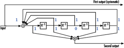
This section explains how to use the Convolutional Encoder block to implement a systematic encoder with feedback. A code is systematic if the actual message words appear as part of the codewords. The following diagram shows an example of a systematic encoder.

Systematic encoder diagram with one input, two outputs and four registers.

To implement this encoder, set the Trellis structure parameter in the Convolutional Encoder block to poly2trellis(5, [37 33], 37). This setting corresponds to

Constraint length: 5
Generator polynomial pair: [37 33]
Feedback polynomial: 37

The feedback polynomial is represented by the binary vector [1 1 1 1 1], corresponding to the upper row of binary digits. These digits indicate connections from the outputs of the registers to the adder. The initial 1 corresponds to the input bit. The octal representation of the binary number 11111 is 37.

To implement a systematic code, set the first generator polynomial to be the same as the feedback polynomial in the Trellis structure parameter of the Convolutional Encoder block. In this example, both polynomials have the octal representation 37.

The second generator polynomial is represented by the binary vector [1 1 0 1 1], corresponding to the lower row of binary digits. The octal number corresponding to the binary number 11011 is 33.

For more information on setting the mask parameters for the Convolutional Encoder block, see Polynomial Description of a Convolutional Code.

Soft-Decision Decoding

This example creates a rate 1/2 convolutional code. It uses a quantizer and the Viterbi Decoder block to perform soft-decision decoding. This description covers these topics:

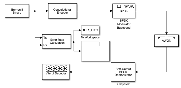
Overview of the Simulation

The simulation creates a random binary message signal, encodes the message into a convolutional code, modulates the code using the binary phase shift keying (BPSK) technique, and adds white Gaussian noise to the modulated data in order to simulate a noisy channel. Then, the simulation prepares the received data for the decoding block and decodes. Finally, the simulation compares the decoded information with the original message signal in order to compute the bit error rate. The Convolutional encoder is configured as a rate 1/2 encoder. For every 2 bits, the encoder adds another 2 redundant bits. To accommodate this, and add the correct amount of noise, the Eb/No (dB) parameter of the AWGN block is in effect halved by subtracting 10*log10(2). The simulation ends after processing 100 bit errors or 10⁷ message bits, whichever comes first.

Simulink model of a BPSK-modulated with convolutional encoding and Viterbi decoding for forward error correction.

Defining the Convolutional Code

The feedforward convolutional encoder in this example is depicted below.

Rate ½ feedforward convolutional encoder with six registers.

While the message data entering the Convolutional Encoder block is a scalar bit stream, the encoded data leaving the block is a stream of binary vectors of length 2.

Mapping the Received Data

Converts the received data signal to a real signal by removing its imaginary part. It is reasonable to assume that the imaginary part of the received data does not contain essential information, because the imaginary part of the transmitted data is zero (ignoring small roundoff errors) and because the channel noise is not very powerful.
Normalizes the received data by dividing by the standard deviation of the noise estimate and then multiplying by -1.
Quantizes the normalized data using three bits.

Decoding the Convolutional Code

Soft-Decision Interpretation of Data

Decision Value	Interpretation
0	Most confident 0
1	Second most confident 0
2	Third most confident 0
3	Least confident 0
4	Least confident 1
5	Third most confident 1
6	Second most confident 1
7	Most confident 1

Traceback and Decoding Delay

The Traceback depth parameter in the Viterbi Decoder block represents the length of the decoding delay. Typical values for a traceback depth are about five or six times the constraint length, which would be 35 or 42 in this example. However, some hardware implementations offer options of 48 and 96. This example chooses 48 because that is closer to the targets (35 and 42) than 96 is.

Delay in Received Data

In this case, the Receive delay value is equal to the Traceback depth value (48).

Comparing Simulation Results with Theoretical Results

This section describes how to compare the bit error rate in this simulation with the bit error rate that would theoretically result from unquantized decoding. The process includes a few steps, described in these sections:

Computing Theoretical Bounds for the Bit Error Rate

To calculate theoretical bounds for the bit error rate P_b of the convolutional code in this model, you can use this estimate based on unquantized-decision decoding:

$P_{b} < \sum_{d = f}^{\infty} c_{d} P_{d}$

In this estimate, c_d is the sum of bit errors for error events of distance d, and f is the free distance of the code. The quantity P_d is the pairwise error probability, given by

$P_{d} = \frac{1}{2} erfc (\sqrt{d R \frac{E_{b}}{N_{0}}})$

where R is the code rate of 1/2, and erfc is the MATLAB complementary error function, defined by

$erfc (x) = \frac{2}{\sqrt{π}} \int_{x}^{\infty} e^{- t^{2}} d t$

Values for the coefficients c_d and the free distance f are in published articles such as "Convolutional Codes with Optimum Distance Spectrum" [3]. The free distance for this code is f = 10.

The following commands calculate the values of P_b for E_b/N₀ values in the range from 1 to 4, in increments of 0.5:

EbNoVec = [1:0.5:4.0];
R = 1/2;
% Errs is the vector of sums of bit errors for
% error events at distance d, for d from 10 to 29.
Errs = [36 0 211 0 1404 0 11633 0 77433 0 502690 0,...
        3322763 0 21292910 0 134365911 0 843425871 0]; 
% P is the matrix of pairwise error probilities, for
% Eb/No values in EbNoVec and d from 10 to 29.
P = zeros(20,7); % Initialize.
for d = 10:29
   P(d-9,:) = (1/2)*erfc(sqrt(d*R*10.^(EbNoVec/10)));
end
% Bounds is the vector of upper bounds for the bit error
% rate, for Eb/No values in EbNoVec.
Bounds = Errs*P;

Simulating Multiple Times to Collect Bit Error Rates

You can efficiently vary the simulation parameters by using the sim (Simulink) function to run the simulation from the MATLAB command line. For example, the following code calculates the bit error rate at bit energy-to-noise ratios ranging from 1 dB to 4 dB, in increments of 0.5 dB. It collects all bit error rates from these simulations in the matrix BERVec. It also plots the bit error rates in a figure window along with the theoretical bounds computed in the preceding code fragment.

In the code sample below, the model name doc_softdecision represents the model described in Overview of the Simulation.

% Plot theoretical bounds and set up figure.
figure;
semilogy(EbNoVec,Bounds,'bo',1,NaN,'r*');
xlabel('Eb/No (dB)'); ylabel('Bit Error Rate');
title('Bit Error Rate (BER)');
l = legend('Theoretical bound on BER','Actual BER');
l.AutoUpdate = 'off';
axis([1 4 1e-5 1]);
hold on;

BERVec = [];
% Make the noise level variable.
set_param('doc_softdecision/AWGN Channel',...
    'EsNodB','EbNodB+10*log10(1/2)');
% Simulate multiple times.
for n = 1:length(EbNoVec)
    EbNodB = EbNoVec(n);
    sim('doc_softdecision',5000000);
    BERVec(n,:) = BER_Data;
    semilogy(EbNoVec(n),BERVec(n,1),'r*'); % Plot point.
    drawnow;
end
hold off;

Note

The estimate for P_b assumes that the decoder uses unquantized data, that is, an infinitely fine quantization. By contrast, the simulation in this example uses 8-level (3-bit) quantization. Because of this quantization, the simulated bit error rate is not quite as low as the bound when the signal-to-noise ratio is high.

The plot of bit error rate against signal-to-noise ratio follows. The locations of your actual BER points might vary because the simulation involves random numbers.

Plot of BER versus Eb/N0 curves to compare theoretical bound to actual BERs.

Tailbiting Encoding Using Feedback Encoders

This example demonstrates Tailbiting encoding using feedback encoders. For feedback encoders, the ending state depends on the entire block of data. To accomplish tailbiting, you must calculate for a given information vector (of N bits), the initial state, that leads to the same ending state after the block of data is encoded.

This is achieved in two steps:

The first step is to determine the zero-state response for a given block of data. The encoder starts in the all-zeros state. The whole block of data is input and the output bits are ignored. After N bits, the encoder is in a state X_N^[zs]. From this state, we calculate the corresponding initial state X₀ and initialize the encoder with X₀.
The second step is the actual encoding. The encoder starts with the initial state X₀, the data block is input and a valid codeword is output which conforms to the same state boundary condition.

Refer to [8] for a theoretical calculation of the initial state X₀ from X_N^[zs] using state-space formulation. This is a one-time calculation which depends on the block length and in practice could be implemented as a look-up table. Here we determine this mapping table by simulating all possible entries for a chosen trellis and block length.

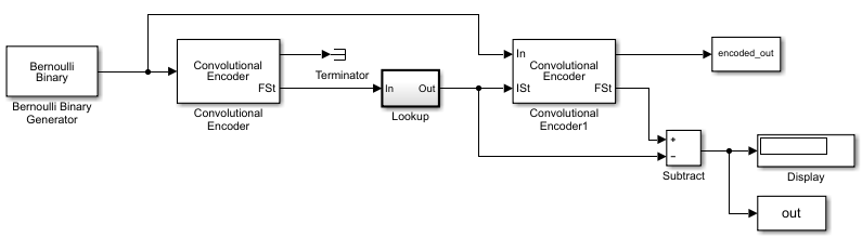
Tailbiting encoding using feedback convolutional encoders.

Assemble blocks to build the model. In the code sample below, the model name doc_mtailbiting_wfeedback represents the model described in the figure.

function mapStValues = getMapping(blkLen, trellis)
% The function returns the mapping value for the given block
length and trellis to be used for determining the initial
state from the zero-state response.

% All possible combinations of the mappings
mapStValuesTab = perms(0:trellis.numStates-1);

% Loop over all the combinations of the mapping entries:
for i = 1:length(mapStValuesTab)
mapStValues = mapStValuesTab(i,:);

% Model parameterized for the Block length
sim('mtailbiting_wfeedback');

% Check the boundary condition for each run
% if ending and starting states match, choose that mapping set
if unique(out)==0
        return
    end
end

Selecting the returned mapStValues for the Table data parameter of the Direct Lookup Table (n-D) block in the Lookup subsystem will perform tailbiting encoding for the chosen block length and trellis.

Selected Bibliography for Convolutional Coding

[1] Clark, George C., and J. Bibb Cain. Error-Correction Coding for Digital Communications. Applications of Communications Theory. New York: Plenum Press, 1981.

[2] Gitlin, Richard D., Jeremiah F. Hayes, and Stephen B. Weinstein. Data Communications Principles. Applications of Communications Theory. New York: Plenum Press, 1992.

[3] Frenger, P., P. Orten, and T. Ottosson. “Convolutional Codes with Optimum Distance Spectrum.” IEEE^® Communications Letters 3, no. 11 (November 1999): 317–19. https://doi.org/10.1109/4234.803468.

Convolutional Codes

Convolutional Code Features

Polynomial Description of a Convolutional Code

Constraint Lengths

Generator Polynomials

Feedback Connection Polynomials

Use Trellis Structure for Rate 1/2 Feedback Convolutional Encoder

Using the Polynomial Description in MATLAB

Trellis Description of a Convolutional Code

Specifying a Trellis in MATLAB

How to Create a MATLAB Trellis Structure

Example: A MATLAB Trellis Structure

Create and Decode Convolutional Codes

Encoding

Hard-Decision Decoding

Soft-Decision Decoding

Implement Soft-Decision Decoding Using Simulink

Design a Rate-2/3 Feedforward Encoder Using MATLAB

Determining Coding Parameters

Using the Encoder

Design a Rate 2/3 Feedforward Encoder Using Simulink

How to Determine Coding Parameters

How to Simulate the Encoder

Notes on the Model

Puncture a Convolutional Code Using MATLAB

Implement a Systematic Encoder with Feedback Using Simulink

Soft-Decision Decoding

Overview of the Simulation

Defining the Convolutional Code

Mapping the Received Data

Decoding the Convolutional Code

Delay in Received Data

Comparing Simulation Results with Theoretical Results

Tailbiting Encoding Using Feedback Encoders

Selected Bibliography for Convolutional Coding

See Also

Topics