Linear-Quadratic-Gaussian (LQG) Design
Linear-quadratic-Gaussian (LQG) control is a modern state-space technique for designing optimal dynamic regulators and servo controllers with integral action (also known as setpoint trackers). This technique allows you to trade off regulation/tracker performance and control effort, and to take into account process disturbances and measurement noise.
To design LQG regulators and setpoint trackers, you perform the following steps:
Construct the LQ-optimal gain.
Construct a Kalman filter (state estimator).
Form the LQG design by connecting the LQ-optimal gain and the Kalman filter.
For more information about using LQG design to create LQG regulators , see Linear-Quadratic-Gaussian (LQG) Design for Regulation.
For more information about using LQG design to create LQG servo controllers, see Linear-Quadratic-Gaussian (LQG) Design of Servo Controller with Integral Action.
These topics focus on the continuous-time case. For information about discrete-time LQG
design, see the dlqr and kalman reference pages.
Linear-Quadratic-Gaussian (LQG) Design for Regulation
You can design an LQG regulator to regulate the output y around zero in the following model.
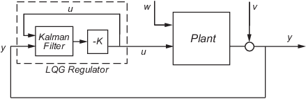
The plant in this model experiences disturbances (process noise) w and is driven by controls u. The regulator relies on the noisy measurements y to generate these controls. The plant state and measurement equations take the form of
and both w and v are modeled as white noise.
Note
LQG design requires a state-space model of the plant. You can use ss to convert other model formats to state space.
To design LQG regulators, you can use the design techniques shown in the following table.
| To design an LQG regulator using... | Use the following commands: |
|---|---|
|
A quick, one-step design technique when the following is true:
| lqg |
|
A more flexible, three-step design technique that allows you to specify:
|
For more information, see
|
Constructing the Optimal State-Feedback Gain for Regulation
You construct the LQ-optimal gain from the following elements:
To construct the optimal gain, type the following command:
K= lqr(A,B,Q,R,N)
This command computes the optimal gain matrix K, for which the
state feedback law minimizes the following quadratic cost function for continuous time:
The software computes the gain matrix K by solving an algebraic Riccati equation.
For information about constructing LQ-optimal gain, including the cost function that
the software minimizes for discrete time, see the lqr reference page.
Constructing the Kalman State Estimator
You need a Kalman state estimator for LQG regulation and servo control because you cannot implement optimal LQ-optimal state feedback without full state measurement.
You construct the state estimate such that remains optimal for the output-feedback problem. You construct the Kalman state estimator gain from the following elements:
Note
You construct the Kalman state estimator in the same way for both regulation and servo control.
To construct the Kalman state estimator, type the following command:
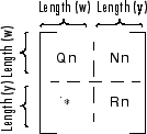
[kest,L,P] = kalman(sys,Qn,Rn,Nn);
This command computes a Kalman state estimator, kest with the
following plant equations:
where w and v are modeled as
white noise. L is the Kalman gain and P the
covariance matrix.
The software generates this state estimate using the Kalman filter
with inputs u (controls) and y (measurements). The noise covariance data
determines the Kalman gain L through an algebraic Riccati equation.
The Kalman filter is an optimal estimator when dealing with Gaussian white noise.
Specifically, it minimizes the asymptotic covariance
of the estimation error .
![]()
For more information, see the kalman reference page. For a complete example of a Kalman filter
implementation, see Kalman
Filtering.
Forming the LQG Regulator
To form the LQG regulator, connect the Kalman filter kest
and LQ-optimal gain K by typing the following
command:
regulator = lqgreg(kest, K);
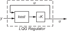
The regulator has the following state-space equations:
For more information on forming LQG regulators, see lqgreg and LQG Regulation: Rolling Mill Case Study.
Linear-Quadratic-Gaussian (LQG) Design of Servo Controller with Integral Action
You can design a servo controller with integral action for the following model:
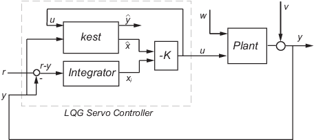
The servo controller you design ensures that the output y tracks the reference command r while rejecting process disturbances w and measurement noise v.
The plant in the previous figure is subject to disturbances w and is driven by controls u. The servo controller relies on the noisy measurements y to generate these controls. The plant state and measurement equations are of the form
and both w and v are modeled as white noise.
Note
LQG design requires a state-space model of the plant. You can use ss to convert other model formats to state space.
To design LQG servo controllers, you can use the design techniques shown in the following table.
| To design an LQG servo controller using... | Use the following commands: |
|---|---|
|
A quick, one-step design technique when the following is true:
| lqg |
|
A more flexible, three-step design technique that allows you to specify:
|
For more information, see
|
Constructing the Optimal State-Feedback Gain for Servo Control
You construct the LQ-optimal gain from the
State-space plant model
sysWeighting matrices
Q,R, andN, which define the tradeoff between tracker performance and control effort
To construct the optimal gain, type the following command:
K= lqi(sys,Q,R,N)
This command computes the optimal gain matrix K, for which the
state feedback law minimizes the following quadratic cost function for continuous time:
The software computes the gain matrix K by solving an algebraic Riccati equation.
For information about constructing LQ-optimal gain, including the cost function that
the software minimizes for discrete time, see the lqi reference page.
Constructing the Kalman State Estimator
You need a Kalman state estimator for LQG regulation and servo control because you cannot implement LQ-optimal state feedback without full state measurement.
You construct the state estimate such that remains optimal for the output-feedback problem. You construct the Kalman state estimator gain from the following elements:
Note
You construct the Kalman state estimator in the same way for both regulation and servo control.
To construct the Kalman state estimator, type the following command:
[kest,L,P] = kalman(sys,Qn,Rn,Nn);
This command computes a Kalman state estimator, kest with the
following plant equations:
where w and v are modeled as
white noise. L is the Kalman gain and P the
covariance matrix.
The software generates this state estimate using the Kalman filter
with inputs u (controls) and y (measurements). The noise covariance data
determines the Kalman gain L through an algebraic Riccati equation.
The Kalman filter is an optimal estimator when dealing with Gaussian white noise.
Specifically, it minimizes the asymptotic covariance
of the estimation error .
![]()
For more information, see the kalman reference page. For a complete example of a Kalman filter
implementation, see Kalman
Filtering.
Forming the LQG Servo Controller
To form a two-degree-of-freedom LQG servo controller, connect the Kalman filter
kest and LQ-optimal gain K by typing the following
command:
servocontroller = lqgtrack(kest, K);
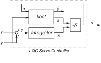
The servo controller has the following state-space equations:
For more information on forming LQG servo controllers, including how to form a
one-degree-of-freedom LQG servo controller, see the lqgtrack reference page.
See Also
lqg | lqr | kalman | lqgtrack | lqi | lqgreg