modalsep
Syntax
Description
[
computes the modal decomposition for a linear time-invariant (LTI) system
H,H0] = modalsep(G)G and returns the modal components as a state-space array
H and the static gain H0.
Each modal component in Hj(s) is associated with a single real pole, a pair of complex conjugate poles, or a cluster repeated poles.
For sparse models, this syntax returns a truncated modal form. By default, the function computes up to 1000 modal components associated with the poles of smallest magnitude. (since R2026a)
[
computes the region-based modal decompositionH,H0] = modalsep(G,N,regionFcn)
Here, the modal components
Hj(s) have their poles in
disjoint regions Rj of the complex plane.
N specifies the number of regions and
regionFcn is the name or a handle to the function that specifies
the partition into N regions.
[
returns the modal decomposition based on the options specified by one or more name-value
arguments. Use these options to control the granularity and accuracy of the
decomposition.H,H0] = modalsep(___,Name=Value)
For sparse models, this syntax returns a subset
of modal components based on the options specified by one or more name-value arguments.
This subset is controlled by the Focus and
MaxOrder options. (since R2026a)
Examples
This example shows how to obtain a modal decomposition for a linear time-invariant (LTI) model using modalsep.
Create a random MIMO state-space model with 20 states.
rng(0)
G = rss(20,2,3);
Obtain the modal decomposition of this model.
[H,H0] = modalsep(G);
Examine the size of H.
size(H)
16x1 array of state-space models.
Each model has 2 outputs, 3 inputs, and between 1 and 2 states.
Typically, the modal components are of order 1 or 2, but can have higher orders in case of cluster of repeated poles.
For this model, modalsep returns the static gain H0 for each I/O pair.
H0
H0 =

  D =
            u1       u2       u3
   y1        0   -1.237  -0.3334
   y2   0.1554   -2.193        0

Static gain.
Model Properties
Additionally, you can obtain the original model back from the modal decomposition using modalsum.
G2 = modalsum(H,H0);
sigma(G,G2,'r--')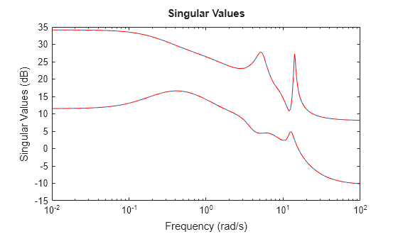
This example shows how to perform region-based modal decomposition of a state-space model. In this example, you perform the modal decomposition of a high-order model based on damping ratio of the poles.
Load a model and examine the damping ratio and natural frequency of the poles.
load('highOrderModel.mat','G')
[wn,zeta] = damp(G);
Visualize the damping ratios and natural frequencies.
semilogy(zeta,wn,"x");
grid on
title("Mode Damping and Natural Frequency")
ylabel("Natural frequency")
xlabel("Damping")

Based on this, you can define regions function that decomposes the model based on the damping ratio values. For example, this model has damping ratios between 0.023 and 0.05, you can divide three regions as follows:
Region 1:
Region 2:
Region 3:
The region function to assign region index to these values is defined at the end of this example. See Region Function Definition.
Perform the modal decomposition.
[h,h0,info] = modalsep(G,3,@regionFcn);
Examine the size of each region.
size(h(:,:,1))
State-space model with 1 outputs, 1 inputs, and 24 states.
size(h(:,:,2))
State-space model with 1 outputs, 1 inputs, and 12 states.
size(h(:,:,3))
State-space model with 1 outputs, 1 inputs, and 12 states.
For this decomposition, region 1 has 24 poles in the specified range. Region 2 and 3 have 12 poles each in their specified ranges.
Region Function Definition
function IR = regionFcn(p)
    [~,z] = damp(p);
    IR = zeros(size(z));
    IR(z<0.033 & z>=0.023) = 1;
    IR(z<0.04 & z>=0.033) = 2;
    IR(z>=0.04) = 3;
end
Since R2026a
This example shows how to obtain a truncated modal decomposition for a sparse model using modalsep.
Load the sparse model.
load flowmeterSparse.mat
size(sys)
Sparse state-space model with 5 outputs, 1 inputs, and 9669 states.
The sparse model contains 9669 states. By default, modalsep computes the first 1000 modal components associated with the poles of smallest magnitude for sparse models, which may be time consuming. Computing the modal decomposition, you can see that modalsep returns an array containing 1000 modal components.
[H,H0,info] = modalsep(sys);
size(H)
1000x1 array of state-space models.
Each model has 5 outputs, 1 inputs, and 1 states.
You can limit the subset of computed modal components using the Focus and MaxOrder options. Compute the modal components in the frequency range 0 rad/s to 250 rad/s and perform region-based modal decomposition to partition modal components in the complex plane. For example, split modal components into two regions:
Region 1 — Poles with absolute value greater than 100.
Region 2 — Poles with absolute value less than 100.
regionFcn = @(p) 1+(abs(p)<100);
N = 2;
[Hr,H0r,infor] = modalsep(sys,N,regionFcn,Focus=[0 250]);
size(Hr)
2x1 array of state-space models.
Each model has 5 outputs, 1 inputs, and between 13 and 20 states.
The function now returns a decomposition with two modal components, with 33 modes split into the specified regions.
Additionally, you can use modalsum to combine the components and obtain a lower-order approximation of the sparse model. The accuracy depends on the number of computed modal components.
sysm = modalsum(H,H0);
sysm2 = modalsum(Hr,H0r);
sigmaplot(sys,sysm,".-",sysm2,"--",w)
legend("Original model","Approximation (1000 poles)",...
    "Approximation (33 poles)")
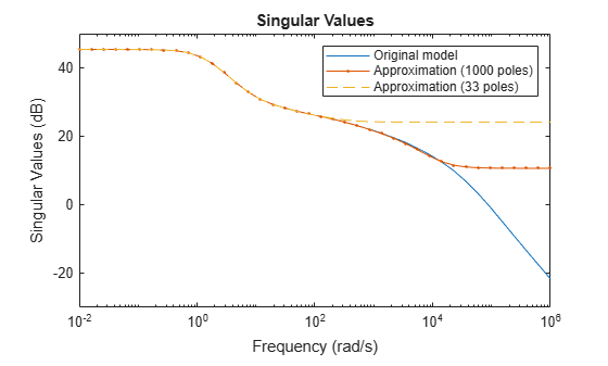
Use this workflow to quickly obtain a truncated modal decomposition of a sparse model. For more flexibility, first use reducespec to obtain a reduced-order model, then apply modalsep to the result.
Input Arguments
Name-Value Arguments
Output Arguments
References
[1] Stewart, G. W. “A Krylov--Schur Algorithm for Large Eigenproblems.” SIAM Journal on Matrix Analysis and Applications 23, no. 3 (January 2002): 601–14. https://doi.org/10.1137/S0895479800371529.