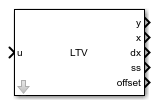
LTV System

Simulate linear time-varying (LTV) systems

Since R2024a

• 

Libraries:
Control System Toolbox / Linear Parameter Varying

Description

A linear time-varying (LTV) system is a linear state-space model whose dynamics vary with time. In MATLAB^®, an LTV model is represented in a state-space form using coefficients that are time dependent.

Mathematically, you can represent an LTV system as follows.

$$\begin{array}{l}dx\left(t\right)=\overline{dx}\left(t\right)+A\left(t\right)\left(x\left(t\right)-\overline{x}\left(t\right)\right)+B\left(t\right)\left(u\left(t\right)-\overline{u}(t)\right)\\ y\left(t\right)=\overline{y}\left(t\right)+C\left(t\right)\left(x\left(t\right)-\overline{x}\left(t\right)\right)+D\left(t\right)\left(u\left(t\right)-\overline{u}(t)\right)\\ x\left(0\right)=x_{init}\end{array}$$

Here,

• u(t) are the inputs

• y(t) are the outputs

• x(t) are the model states with initial value x_init

• $dx\left(t\right)$ is the state derivative vector $\dot{x}$ for continuous-time systems and the state update vector x[k+1] for discrete-time systems. Here, k is the integer index that counts the number of sampling periods T_s.

• A(t), B(t), C(t), and D(t) are the state-space matrices dependent of time t.

• dx₀(t), x₀(t), u₀(t), and y₀(t) are the offsets in the values of $dx\left(t\right)$, x(t), u(t) and y(t) at a given time t.

  You can obtain the offsets by returning additional linearization information when calling functions such as linearize (Simulink Control Design) or getIOTransfer (Simulink Control Design).

The block accepts an array of state-space models with operating point information. The block extracts the time dependence information from the SamplingGrid property of the LTI array and picks the local dynamics from this operating space. The block uses this array with data interpolation and extrapolation techniques for simulation.

You can obtain the offsets by returning additional linearization information when calling functions such as linearize (Simulink Control Design) or getIOTransfer (Simulink Control Design).

Examples

Create and Simulate Linear Time-Varying Model Using LTV System Block

This example shows how to simulate a linear time-varying (LTV) model using the LTV System block. The LTV System block interpolates a state-space array to model the LTV response. In this example, you batch linearize the model defined by the following equation at time snapshots to obtain the array of linear state-space models.

$$\dot{\mathit{x}}=\frac{-1}{1+\mathit{t}}\mathit{x}$$

Open the model.

mdl = 'nonLinModel';
open_system(mdl);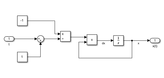

Specify the initial condition.

xinit = 10;

Simulate the model and extract operating points at time snapshots.

tlin = logspace(-1,log10(30),20);
op = findop(mdl,tlin);

Specify model linear analysis points.

io(1) = linio('nonLinModel/Ramp',1,'input');
io(2) = linio('nonLinModel/Plant',1,'output');

Compute the linearizations along with offsets.

opt = linearizeOptions('StoreOffsets',true);
[linsys,~,info] = linearize(mdl,op,io,opt);
linsys.SamplingGrid = struct('Time',tlin);

This linearization result is a state-space array of the system.

size(linsys)

20x1 array of state-space models.
Each model has 1 outputs, 1 inputs, and 1 states.

You can now use this array with the LTV System block.

Open the CompareNLandLTV model. This model contains the preconfigured LTV block.

ltvMdl = "CompareNLandLTV";
open_system(ltvMdl)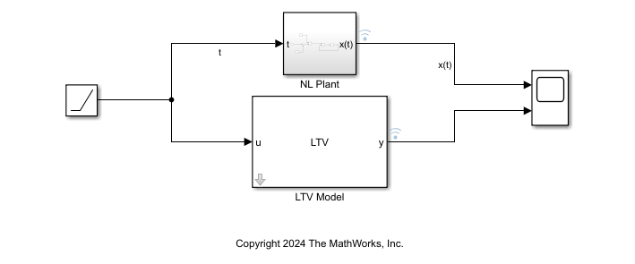

Simulate the LTV model and compare the results.

out = sim(ltvMdl);
plot(out.logsout{2}.Values.Time,out.logsout{2}.Values.Data,...
    out.logsout{1}.Values.Time,out.logsout{1}.Values.Data,"r--")
legend("Nonlinear model","LTV model")
grid on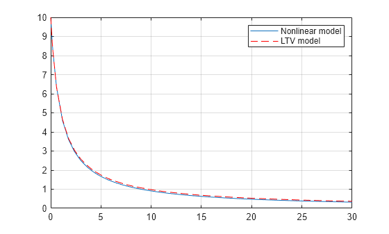

The LTV model provides a good approximation for the nonlinear model simulation.

Close the models.

close_system(mdl,0);
close_system(ltvMdl,0);

Limitations

• Internal delays cannot be extrapolated to be less than their minimum value in the state-space model array.

Ports

Input

u — Input signal

scalar | vector

Specify the input signal u(t). In multi-input case, this port accepts a signal of the dimension of the input.

Output

y — Model output

scalar | vector

Response of the linear time-varying model.

x — State values

scalar | vector

Values of the model states

Dependencies

To enable this port, select Output states on the Outputs tab of the block parameters.

dx — State derivative values

scalar | vector

Values of the state derivatives.

Dependencies

To enable this port, select Output state derivatives (continuous-time) or updates (discrete-time) on the Outputs tab of the block parameters.

ss — Local state-space model

bus

Local state-space model data at the major simulation time steps, returned as a bus signal with these elements.

• A — State matrix

• B — Input matrix

• C — Output matrix

• D — Feedthrough matrix

• InputDelay — Input delay

• OutputDelay — Output delay

• InternalDelay — Internal delays in the model

Dependencies

To enable this port, select Output interpolated state-space data on the Outputs tab of the block parameters.

offset — LPV model offsets

bus

LTV model offset data at the major simulation time steps, returned as a bus signal with these elements.

• InputOffset

• OutputOffset

• StateOffset

• StateDerivativeOffset

Dependencies

To enable this port, select Output interpolated offsets on the Outputs tab of the block parameters.

Parameters

To edit block parameters interactively, use the Property Inspector. From the Simulink^® Toolstrip, on the Simulation tab, in the Prepare gallery, select Property Inspector.

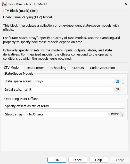
LTV Model Tab

State-space array — Array of state-space models

ss or idss model array

An array of state-space (ss or idss (System Identification Toolbox)) models. All the models in the array must use the same definition of states.

The state-space array must specify the dependence on time in the SamplingGrid property. You can also specify the model offsets in the Offsets property of the array when you set the Operating Point Offsets parameter to Use offsets in state-space array, See the ss model reference page for more information on these properties.

When the block is in a model with synchronous state control (see the State Control (HDL Coder) block), you must specify an array of discrete-time models.

Programmatic Use

To set the block parameter value programmatically, use the set_param (Simulink) function.

Parameter:	sys
Values:	ss or idss model array name in quotes

Example: set_param(gcb,"sys","sysArrayName")

Initial state — Initial conditions

0 (default) | vector

Initial conditions to use with the local model to start the simulation, specified as a vector of length equal to the number of model states.

Programmatic Use

To set the block parameter value programmatically, use the set_param (Simulink) function.

Parameter:	x0
Values:	"0" (default) | initial state values in quotes

Example: set_param(gcb,"x0","[0 0.1]")

Operating Point Offsets — Offset specification format

Specify Offsets as double arrays (default) | Specify offsets as struct array | Use offsets in state-space array

Specify the format for operating point offsets.

• Specify Offsets as double arrays — Specify offsets using the Input offset, Output offset, State Offset, and State derivative/update offset parameters.

• Specify offsets as struct array — Specify offsets as a structure array with fields u, y, x, and dx specifying the input, output, state, and state derivative offsets, respectively.

• Use offsets in state-space array — Use the offsets specified in the Offsets property of the state-space array.

Programmatic Use

To set the block parameter value programmatically, use the set_param (Simulink) function.

Parameter:	opSpecOption
Values:	"Specify Offsets as double arrays" (default) | "Specify offsets as struct array" | "Use offsets in state-space array"

Example: set_param(gcb,"opSpecOption","Specify offsets as struct array")

Input offset — Input offset

0 (default) | array

Offsets in input u(t), specified as one of the following:

• 0 — Use when there are no input offsets.

• Double vector of length equal to the number of inputs — Use when input offset is the same across the scheduling space.

• Double array of size n_u-by-1-by-N — Use when offsets are present and they vary across the scheduling space. Here, n_u is the number of inputs and N is the number of time snapshots. For example, if your model has three inputs, two outputs, and four states and is scheduled over 10 time snapshots, the array size must be 3-by-1-by-10. Use size(sys) to determine the size of the state-space array sys.

Dependencies

To enable this parameter, set the Operating Point Offsets format to Specify Offsets as double arrays

Programmatic Use

To set the block parameter value programmatically, use the set_param (Simulink) function.

Parameter:	uOffset
Values:	"0" (default) | array name in quotes

Example: set_param(gcb,"uOffset","uOffArray")

Output offset — Output offset

0 (default) | array

Offsets in output y(t), specified as one of the following:

• 0 Use when there are no output offsets.

• Double vector of length equal to the number of outputs. Use when output offsets are the same across the scheduling space.

• Double array of size n_y-by-1-by-N — Use when offsets are present and they vary across the scheduling space. Here, n_y is the number of outputs and N is the number of time snapshots. For example, if your model has three inputs, two outputs, and four states and is scheduled over 10 time snapshots, the array size must be 2-by-1-by-10. Use size(sys) to determine the size of the state-space array sys.

Dependencies

To enable this parameter, set the Operating Point Offsets format to Specify Offsets as double arrays

Programmatic Use

To set the block parameter value programmatically, use the set_param (Simulink) function.

Parameter:	yOffset
Values:	"0" (default) | array name in quotes

Example: set_param(gcb,"yOffset","yOffArray")

State offset — State offset

0 (default) | array

Offsets in states x(t), specified as one of the following:

• 0 — Use when there are no state offsets.

• Double vector of length equal to the number of states — Use when the state offsets are the same across the scheduling space.

• Double array of size n_x-by-1-by-N — Use when offsets are present and they vary across the scheduling space. Here, n_x is the number of states and N is the number of time snapshots. For example, if your model has three inputs, two outputs, and four states and is scheduled over 10 time snapshots, the array size must be 4-by-1-by-10. Use size(sys) to determine the size of the state-space array sys.

Dependencies

To enable this parameter, set the Operating Point Offsets format to Specify Offsets as double arrays

Programmatic Use

To set the block parameter value programmatically, use the set_param (Simulink) function.

Parameter:	xOffset
Values:	"0" (default) | array name in quotes

Example: set_param(gcb,"xOffset","xOffArray")

State derivative/update offset — State derivative or update offset

array

Offsets in state derivative or update variable dx(t), specified as one of the following:

• If you obtained the linear system array by linearization under equilibrium conditions, select the Assume equilibrium operating conditions option. This option corresponds to an offset of $$\overline{dx}(t)=0$$ for a continuous-time system and $$\overline{dx}(t)=\overline{x}(t)$$ for a discrete-time system. This option is selected by default.

• If the linear system contains at least one system that you obtained under non-equilibrium conditions, clear the Assume equilibrium operating conditions option. Specify one of the following in the Offset value field:

  • If the dx offset values are the same across the scheduling space, specify as a double vector of length equal to the number of states.

  • If the dx offsets are present and they vary across the scheduling space, specify as a double array of size n_x-by-1-by-N — Use when offsets are present and they vary across the scheduling space. Here, n_x is the number of states and N is the number of time snapshots. For example, if your model has three inputs, two outputs, and four states and is scheduled over 10 time snapshots, the array size must be 4-by-1-by-10. Use size(sys) to determine the size of the state-space array sys.

Dependencies

To enable this parameter, set the Operating Point Offsets format to Specify Offsets as double arrays and disable Assume equilibrium operating conditions.

Programmatic Use

To set the block parameter value programmatically, use the set_param (Simulink) function.

Parameter:	dxOffset
Values:	"0" (default) | array name in quotes

Example: set_param(gcb,"dxOffset","dxOffArray")

Struct array — Offsets structure array

struct (default) | structure array name

Model offsets, specified as a structure with these fields.

Field	Description
u	Input offsets
y	Output offsets
x	State offsets
dx	State derivative offsets

• If offset values are the same across the scheduling space, specify as a double vector of length equal to the number of inputs, outputs, or states for the corresponding fields.

• If the offsets vary across scheduling space, specify a multidimensional array for each field. For instance, suppose that your model has three inputs, two outputs, and four states. If you linearize your model using a 5-by-6 array of operating points, the structure array size must be 5-by-6 and each entry must contain a vector of length equal to the number of inputs, outputs, or states for the corresponding fields.

The linearize (Simulink Control Design) function returns offsets in this format in the info.Offsets output when you linearize with StoreOffsets option set to true.

Dependencies

To enable this parameter, set the Operating Point Offsets format to Specify Offsets as struct array

Programmatic Use

To set the block parameter value programmatically, use the set_param (Simulink) function.

Parameter:	Offset
Values:	"struct" (default) | structure array name in quotes

Example: set_param(gcb,"Offset","OffsetStructName")

Fixed Entries Tab

Nominal model — Nominal LTV model

Use the first model in state-space array (default) | Custom value

State-space model that provides the values of the fixed coefficients, specified as one of the following:

• Use the first model in state-space array — The first model in the state-space array is used to represent the LTV model. In the following example, the state-space array is specified by object sys and the fixed coefficients are taken from model sys(:,:,1).

  % Specify a 5-by-1 array of state-space models.
  sys = rss(4,2,3,5,1);
  t = 1:5; 
  % Use "Time" as scheduling parameter.
  sys.SamplingGrid = struct("Time",t);  

  Fixed coefficients are taken from the model sysFixed = sys(:,:,1), which corresponds to [Time=1]. If the (2,1) entry of A matrix is forced to be fixed, its value used during the simulation is sysFixed.A(2,1).

• Custom value — Specify a different state-space model for fixed entries. Specify a variable for the fixed model in the State space model field. The fixed model must use the same state basis as the state-space array in the LTV model.

Fixed Coefficient Indices — Fixed coefficients of state-space matrices

false or 0 (default) | true or 1 | logical matrix

Specify which coefficients of the state-space matrices and delay vectors are fixed.

Specify one of the following:

• Scalar Boolean (true or false), if all entries of a matrix are to be treated the same way.

  The default value is false for the state-space matrices and delay vectors, which means that they are treated as free.

• Logical matrix of a size compatible with the size of the corresponding matrix:

  State-space matrix	Size of fixed entry matrix
  A matrix	nx-by-nx
  B matrix	nx-by-nu
  C matrix	ny-by-nx
  D matrix	ny-by-nu
  Input delay	nu-by-1
  Output delay	ny-by-1
  Internal delay	ni-by-1

  where, n_u is the number of inputs, n_y is the number of outputs, n_x is the number of states, n_i is the length of internal delay vector.

• Numerical indices to specify the location of fixed entries. See sub2ind reference page for more information on how to generate numerical indices corresponding to a given subscript (i,j) for an element of a matrix.

Scheduling Tab

Interpolation method — Interpolation method

Linear (default) | Nearest | Flat

Interpolation method. Defines how the state-space data must be computed for scheduling parameter values that are located away from their grid locations.

Specify one of the following options:

• Flat — Choose the state-space data at the grid point closest, but not larger than, the current point. The current point is the value of the scheduling parameters at current time.

• Nearest — Choose the state-space data at the closest grid point in the scheduling space.

• Linear — Obtain state-space data by linear interpolation of the nearest 2d neighbors in the scheduling space, where d = number of scheduling parameters.

The default interpolation scheme is Linear for regular grids of scheduling parameter values. For irregular grids, the Nearest interpolation scheme is always used regardless of the choice you made. To learn more about regular and irregular grids, see Regular vs. Irregular Grids.

The Linear method provides the highest accuracy but takes longer to compute. The Flat and Nearest methods are good for models that have mode-switching dynamics.

Programmatic Use

To set the block parameter value programmatically, use the set_param (Simulink) function.

Parameter:	IMethod
Values:	"Linear" (default) | "Nearest" | "Flat"

Example: set_param(gcb,"IMethod","Flat")

Extrapolation method — Extrapolation method

Clip (default) | Linear

Extrapolation method. Defines how to compute the state-space data for scheduling parameter values that fall outside the range over which the state-space array has been provided (as specified in the SamplingGrid property).

Specify one of the following options:

• Clip (default) — Disables extrapolation and returns the data corresponding to the last available scheduling grid point that is closest to the current point.

• Linear — Fits a line between the first or last pair of values for each scheduling parameter, depending upon whether the current value is less than the first or greater than the last grid point value, respectively. This method returns the point on that line corresponding to the current value. Linear extrapolation requires that the interpolation scheme be linear too.

Programmatic Use

To set the block parameter value programmatically, use the set_param (Simulink) function.

Parameter:	EMethod
Values:	"Clip" (default) | "Linear"

Example: set_param(gcb,"EMethod","Linear")

Index search method — Prelookup algorithm

Binary search (default) | Linear search

The block determines the location of the current scheduling parameter values in the scheduling space using a prelookup algorithm. Select Linear search or Binary search. Each search method has speed advantages in different situations. For more information on this parameter, see the Prelookup (Simulink) block reference page.

Programmatic Use

To set the block parameter value programmatically, use the set_param (Simulink) function.

Parameter:	IndexSearch
Values:	"Binary Search" (default) | "Linear Search"

Example: set_param(gcb,"IndexSearch","Linear Search")

Begin index search using previous index result — Begin search at previous time step

on (default) | off

Select this check box when you want the block to start its search using the index found at the previous time step. For more information on this parameter, see the Prelookup (Simulink) block reference page.

Programmatic Use

To set the block parameter value programmatically, use the set_param (Simulink) function.

Parameter:	IndexBegin
Values:	"on" (default) | "off"

Example: set_param(gcb,"IndexBegin","off")

Code Generation Tab

Block data type (discrete-time case only) — Block data type

double (default) | single

Block data type, specified as double or single.

Dependencies

To enable this option, use a discrete-time state-space model as input.

Programmatic Use

To set the block parameter value programmatically, use the set_param (Simulink) function.

Parameter:	DataType
Values:	"double" (default) | "single"

Example: set_param(gcb,"DataType","single")

Initial buffer size for delays — Initial buffer size

1024 (default) | positive integer greater than 5

Initial memory allocation for the number of input points to store for models that contain delays. If the number of input points exceeds the initial buffer size, the block allocates additional memory. The default size is 1024.

When you run the model in Accelerator mode or build the model, make sure the initial buffer size is large enough to handle maximum anticipated delay in the model.

Programmatic Use

To set the block parameter value programmatically, use the set_param (Simulink) function.

Parameter:	InitBufferSize
Values:	"1024" (default) | positive integer greater than 5 in quotes

Example: set_param(gcb,"InitBufferSize","512")

Use fixed buffer size — Use fixed buffer size

off (default) | on

Specify whether to use a fixed buffer size to save delayed input and output data from previous time steps. Use this option for continuous-time LTV systems that contain input or output delays. If the buffer is full, new data replaces data already in the buffer. The software uses linear extrapolation to estimate output values that are not in the buffer.

Programmatic Use

To set the block parameter value programmatically, use the set_param (Simulink) function.

Parameter:	FixedBuffer
Values:	"off" (default) | "on"

Example: set_param(gcb,"FixedBuffer","on")

Extended Capabilities

C/C++ Code Generation
Generate C and C++ code using Simulink® Coder™.

Version History

Introduced in R2024a