info
Information about filter System object
Description
Examples
Obtain short-format and long-format information about a filter.
d = fdesign.lowpass;
f = design(d,SystemObject=true);
info(f)
ans = 7×35 char array
    'Discrete-Time FIR Filter (real)    '
    '-------------------------------    '
    'Filter Structure  : Direct-Form FIR'
    'Filter Length     : 43             '
    'Stable            : Yes            '
    'Linear Phase      : Yes (Type 1)   '
    'Input sample rate : Normalized     '
info(f,'long')ans = 46×45 char array
'Discrete-Time FIR Filter (real) '
'------------------------------- '
'Filter Structure : Direct-Form FIR '
'Filter Length : 43 '
'Stable : Yes '
'Linear Phase : Yes (Type 1) '
' '
'Design Method Information '
'Design Algorithm : equiripple '
' '
'Design Options '
'Density Factor : 16 '
'Maximum Phase : false '
'Minimum Order : any '
'Minimum Phase : false '
'Stopband Decay : 0 '
'Stopband Shape : flat '
'SystemObject : true '
'Uniform Grid : true '
' '
'Design Specifications '
'Sample Rate : N/A (normalized frequency) '
'Response : Lowpass '
'Specification : Fp,Fst,Ap,Ast '
'Passband Edge : 0.45 '
'Stopband Edge : 0.55 '
'Passband Ripple : 1 dB '
'Stopband Atten. : 60 dB '
' '
'Measurements '
'Sample Rate : N/A (normalized frequency)'
'Passband Edge : 0.45 '
'3-dB Point : 0.46957 '
'6-dB Point : 0.48314 '
'Stopband Edge : 0.55 '
'Passband Ripple : 0.89042 dB '
'Stopband Atten. : 60.945 dB '
'Transition Width : 0.1 '
' '
'Implementation Cost '
'Number of Multipliers : 43 '
'Number of Adders : 42 '
'Number of States : 42 '
'Multiplications per Input Sample : 43 '
'Additions per Input Sample : 42 '
'Input sample rate : Normalized '
Decimate a signal from 44.1 kHz to 11.025 kHz using a dsp.CICDecimator System object™ with DecimationFactor set to 4. Begin by creating the dsp.CICDecimator object.
cicdec = dsp.CICDecimator(DecimationFactor=4, ...
    FixedPointDataType="Minimum section word lengths", ...
    OutputWordLength=16);
Construct a 1 kHz sinusoidal generator with a sample rate of 44.1 kHz and 64 samples per frame.
FsIn = 44.1e3;
sine = dsp.SineWave(Frequency=1e3,SampleRate=FsIn,SamplesPerFrame=64);
The input signal for the CIC decimator is a sine wave quantized to a signed fixed-point format with a word length of 16 bits and a fractional length of 15 bits.
inDT = numerictype(true,16,15);
src  = @()fi(sine(),inDT);
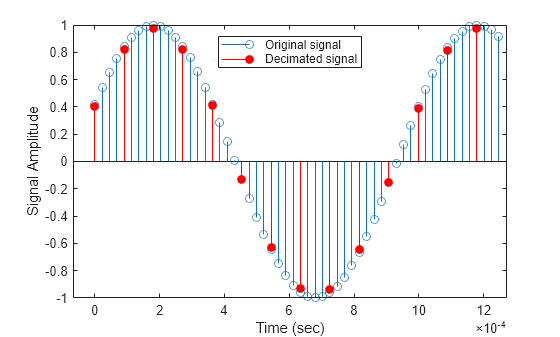
Decimate the input with a factor of 4 to obtain 16 samples per output frame. Use the gain function to compute the CIC filter gain. Use the outputDelay function to obtain the CIC latency rate and the output sample rate. Plot the output frames of the original and decimated signals using the parameters you computed.
% Determine the CIC gain
cicGain = gain(cicdec);

% Determine the CIC latency and the output sample rate
[cicDelay,FsOut] = outputDelay(cicdec,InputSampleRate=FsIn);

ts = timescope(NumInputPorts=2, ...
    SampleRate=[FsIn FsOut], ...
    TimeDisplayOffset=[0,-cicDelay], ...
    ChannelNames=["Input signal","Decimated signal"], ...
    YLimits=[-2 2], ...
    PlotType="stem");

for ii = 1:16
    u = src();        % Fetch an input frame
    y = cicdec(u);    % decimate
    ts(u, y/cicGain);
end
Using the info method in "long" format, obtain the word lengths and fraction lengths of the fixed-point filter sections and the filter output.
info(cicdec,"long")ans = 17×56 char array
'Discrete-Time FIR Multirate Filter (real) '
'----------------------------------------- '
'Filter Structure : Cascaded Integrator-Comb Decimator'
'Decimation Factor : 4 '
'Differential Delay : 1 '
'Number of Sections : 2 '
'Stable : Yes '
'Linear Phase : Yes (Type 1) '
' '
' '
'Implementation Cost '
'Number of Multipliers : 0 '
'Number of Adders : 4 '
'Number of States : 4 '
'Multiplications per Input Sample : 0 '
'Additions per Input Sample : 2.5 '
'Input sample rate : Normalized '
Create a dsp.CICInterpolator System object™ with InterpolationFactor set to 2. Interpolate a fixed-point signal by a factor of 2 from 22.05 kHz to 44.1 kHz.
cicint = dsp.CICInterpolator(InterpolationFactor=2)
cicint =
  dsp.CICInterpolator with properties:

    InterpolationFactor: 2
      DifferentialDelay: 1
            NumSections: 2
     FixedPointDataType: 'Full precision'
Create a dsp.SineWave object with SampleRate set to 22.05 kHz, SamplesPerFrame set to 32, and OutputDataType set to "Custom". To generate a fixed-point signal, set the CustomOutputDataType property to a numerictype object. For the purpose of this example, set the value to numerictype([],16). The fraction length is computed based on the values of the generated sinusoidal signal to give the best possible precision.
To generate a fixed-point signal, set the Method property of the dsp.SineWave object to "Table lookup". This method of generating the sinusoidal signal requires that the period of every sinusoid in the output be evenly divisible by the sample period. That is, must be an integer value for every channel i = 1, 2, ..., N. The value of equals , the variable is the frequency of the sinusoidal signal, and is the sample rate of the signal. In other words, the ratio must be an integer. For more details, see the Algorithms section on the dsp.SineWave object page.
In this example, is set to 22050 Hz and is set to 1050 Hz.
FsIn = 22.05e3;
sine = dsp.SineWave(Frequency=1050,...
    SampleRate=FsIn,...
    SamplesPerFrame=32,...
    Method="Table lookup",...
    OutputDataType="Custom",...
    CustomOutputDataType=numerictype([],16));
The output of the CIC interpolation filter is amplified by a specific gain value. You can determine this value using the gain function. This gain equals the gain of the stage of the CIC interpolation filter and equals , where is the interpolation factor, is the differential delay, and is the number of sections of the CIC interpolator.
cicGain = gain(cicint)
cicGain =
2
To adjust this amplified output and to match it to the amplitude of the original signal, divide the CIC interpolated signal with the computed gain value.
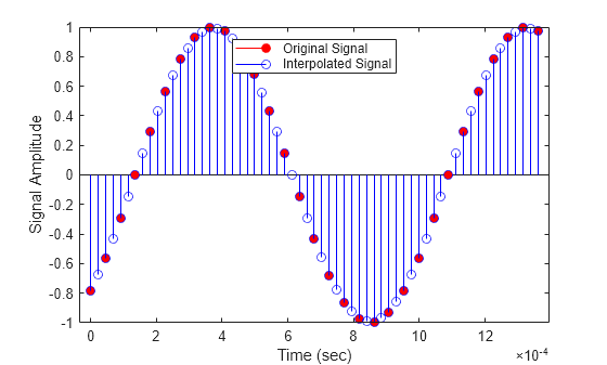
Stream the fixed-point sinusoidal signal of sample rate 22.05 kHz. Interpolate each input frame by a factor of 2, producing an interpolated output frame with 64 samples. Plot the original and the interpolated signals, accounting for the CIC interpolation latency and gain.
% Determine the CIC latency and the output sample rate
[cicDelay,FsOut] = outputDelay(cicint,InputSampleRate=FsIn);

ts = timescope(NumInputPorts=2, ...
    SampleRate=[FsOut FsIn], ...
    TimeDisplayOffset=[0,cicDelay], ...
    ChannelNames=["Interpolated signal","Input signal"], ...
    YLimits=[-2 2], ...
    PlotType="stem"...
    );

for i = 1:16
    % Fetch an input frame and interpoalte it
    u = sine();
    y = cicint(u);
    ts(y/cicGain,u);
end
Using the info function in the "long" format, obtain the word lengths and fraction lengths of the fixed-point filter sections and the filter output.
info(cicint,"long")ans = 17×61 char array
'Discrete-Time FIR Multirate Filter (real) '
'----------------------------------------- '
'Filter Structure : Cascaded Integrator-Comb Interpolator'
'Interpolation Factor : 2 '
'Differential Delay : 1 '
'Number of Sections : 2 '
'Stable : Yes '
'Linear Phase : Yes (Type 1) '
' '
' '
'Implementation Cost '
'Number of Multipliers : 0 '
'Number of Adders : 4 '
'Number of States : 4 '
'Multiplications per Input Sample : 0 '
'Additions per Input Sample : 6 '
'Input sample rate : Normalized '
Since R2026a
Using SampleRate Argument
Specify the input sample rate explicitly while constructing the dsp.FIRFilter object using the SampleRate argument.
firFilt = dsp.FIRFilter(SampleRate=22050)
firFilt =
  dsp.FIRFilter with properties:

            Structure: 'Direct form'
      NumeratorSource: 'Property'
            Numerator: [0.5000 0.5000]
    InitialConditions: 0

  Show all properties
You can view this information using the Input sample rate field of the info function.
info(firFilt)
ans = 7×35 char array
    'Discrete-Time FIR Filter (real)    '
    '-------------------------------    '
    'Filter Structure  : Direct-Form FIR'
    'Filter Length     : 2              '
    'Stable            : Yes            '
    'Linear Phase      : Yes (Type 2)   '
    'Input sample rate : 22050          '
Visualize the frequency response of the filter using filterAnalyzer. Note the frequency range from 0 to 11025 Hz.
filterAnalyzer(firFilt,FilterNames="FIRFilter22050Hz")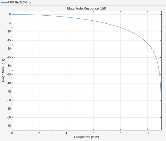
Using setInputSampleRate Function
To specify the input sample rate after constructing the object, use the setInputSampleRate function.
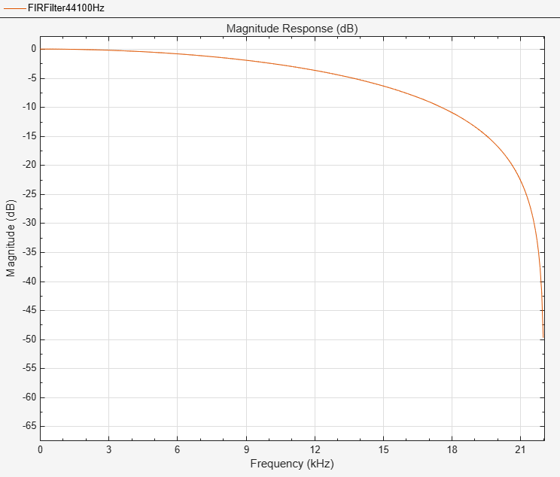
setInputSampleRate(firFilt,44100)
To confirm, view the sample rate information using the info function.
info(firFilt)
ans = 7×35 char array
    'Discrete-Time FIR Filter (real)    '
    '-------------------------------    '
    'Filter Structure  : Direct-Form FIR'
    'Filter Length     : 2              '
    'Stable            : Yes            '
    'Linear Phase      : Yes (Type 2)   '
    'Input sample rate : 44100          '
Visualize the frequency response of the filter using filterAnalyzer. Note the change in frequency interval from 0 to 22050 Hz.
filterAnalyzer(firFilt,FilterNames="FIRFilter44100Hz")