dsp.FourthOrderSectionFilter
R2026bImplement cascade of fourth-order section filters
Description
The dsp.FourthOrderSectionFilter object implements a cascade of
fourth-order section filters.
Creation
Syntax
Description
fos = dsp.FourthOrderSectionFilterFourthOrderSectionFilter object, fos, that
implements a cascade of fourth-order filter sections.
fos = dsp.FourthOrderSectionFilter(num,den)FourthOrderSectionFilter object with the
Numerator property set to num and the
Denominator property set to den.
fos = dsp.FourthOrderSectionFilter(___,SampleRate=Value)"normalized". (since R2026a)
To specify an input sample rate of 22050 Hz, set
SampleRate to 22050. To specify the input sample rate in normalized
units, set SampleRate to "normalized". (since R2026a)
fos = dsp.FourthOrderSectionFilter(___,PropertyName=Value)Numerator to a row
vector or a matrix.
Properties
Usage
Syntax
Description
Input Arguments
Output Arguments
Object Functions
Examples
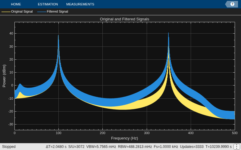
Filter a noisy sinusoidal signal using the dsp.FourthOrderSectionFilter object. Visualize the original and filtered signals using a spectrum analyzer.
Input Signal
The input signal is the sum of two sine waves with frequencies 100 Hz and 350 Hz. Add zero-mean white Gaussian noise with a standard deviation of 1e-4 to the sum of sine waves. The sample rate is 1000 Hz.
frameSize = 1024;
fs = 1000;
Sine1 = dsp.SineWave(5,100,SamplesPerFrame=1024,SampleRate=fs);
Sine2 = dsp.SineWave(2,350,pi/2,SamplesPerFrame=1024,...
    SampleRate=fs);
x = Sine1()+Sine2()+1e-4.*randn(Sine1.SamplesPerFrame,1);
Fourth-Order Section (FOS) Filter Coefficients
The numerator and denominator coefficients for the FOS filter are obtained using designParamEq which is part of Audio Toolbox:
%N = [2,4];
%gain = [5,10];
%centerFreq = [0.025,0.75];
%bandwidth = [0.025,0.35];
%mode = 'fos';
%[num,den] = designParamEQ(FilterOrder=N,Gain=gain,...
% CenterFrequency=centerFreq,Bandwidth=bandwidth,CascadeSectionsForm=mode,...
% Orientation="row");

num = [1.0223   -1.9368    0.9205         0         0
    1.5171    2.3980    1.4317    0.6416    0.2752];

den = [1.0000    -1.9368    0.9428         0         0
    1.0000    2.0136    1.9224    1.0260    0.3016];
Initialize Filter and Spectrum Analyzer
Construct the FOS IIR filter using the num and den coefficients. Construct a spectrum analyzer to visualize the original sinusoidal signal and the filtered signal.
fos = dsp.FourthOrderSectionFilter(Numerator=num,...
    Denominator=den);

scope = spectrumAnalyzer(...
    SampleRate=fs,...
    PlotAsTwoSidedSpectrum=false,...
    FrequencyScale="linear",...
    Method="welch",...
    Title="Original and Filtered Signals",...
    ShowLegend=true,...
    ChannelNames={"Original Signal","Filtered Signal"});
Filter the input signal, and visualize the original and filtered spectrums.
for i = 1:10000
    y = fos(x);
    scope([x,y]);
end
release(scope);
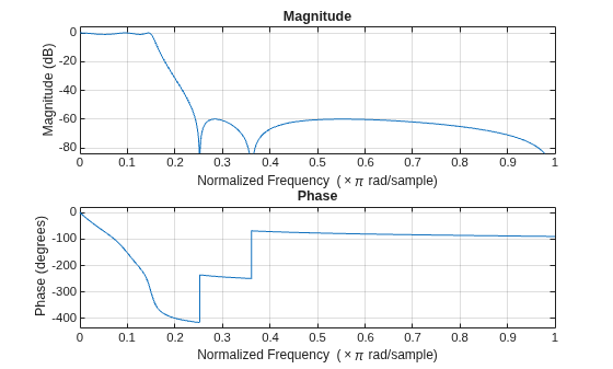
Design a lowpass fourth-order section (FOS) filter using the fdesign function. Using this filter, filter a noisy sinusoidal signal with two tones, one at 3 kHz, and the other at 12 kHz.
Design a fifth-order filter using the elliptic method in the "df2tsos" structure. Use L-infinity norm scaling in the frequency domain. Specify the passband frequency to be 0.15 rad/sample and the stopband frequency to be 0.25 rad/sample. Specify 1 dB of allowable passband ripple and a stopband attenuation of 60 dB.
Fp = 0.15;
Fst = 0.25;
Ap = 1;
Ast = 60;
The filter coefficients are scaled using an fdopts.sosscaling object. The scaling object is defined to have no numerator constraints, and the ScaleValueConstraint is set to "unit", specifying the scaling to be unity scaling.
fdo = fdopts.sosscaling;
fdo.NumeratorConstraint="none";
fdo.ScaleValueConstraint="unit";

f = fdesign.lowpass("Fp,Fst,Ap,Ast",Fp,Fst,Ap,Ast);
hFilter = design(f,"ellip",SystemObject=true,...
    FilterStructure="df2tsos",SOSScaleNorm="Linf",...
    SOSScaleOpts=fdo)
hFilter =
  dsp.SOSFilter with properties:

            Structure: 'Direct form II transposed'
    CoefficientSource: 'Property'
            Numerator: [3×3 double]
          Denominator: [3×3 double]
       HasScaleValues: true
          ScaleValues: [1 1 1 1.0000]

  Show all properties
Visualize the lowpass frequency response of the designed filter.
freqz(hFilter)
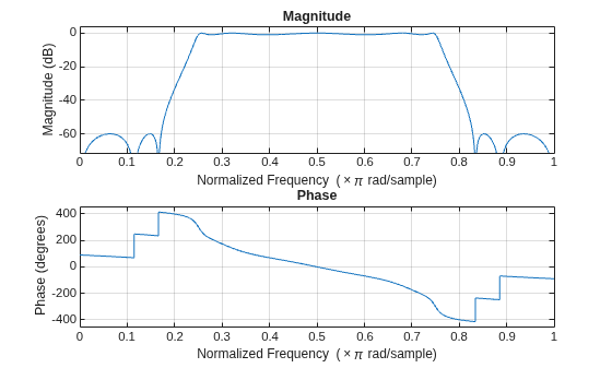
Convert the lowpass filter to a bandpass filter using the iirlp2bp function.
[num,den] = iirlp2bp(hFilter.Numerator,hFilter.Denominator,Fp,[0.25,0.75])
num = 3×5

    0.2456         0   -0.2456         0         0
    0.4175   -0.0000   -0.4206   -0.0000    0.4175
    0.4281   -0.0000   -0.6433   -0.0000    0.4281
den = 3×5

    1.0000   -0.0000    0.5088         0         0
    1.0000   -0.0000    0.0060   -0.0000    0.8657
    1.0000   -0.0000    0.5160   -0.0000    0.5283
Create a fourth-order section filter using these numerator and denominator coefficients.
fos = dsp.FourthOrderSectionFilter(num,den)
fos =
  FourthOrderSectionFilter with properties:

               Numerator: [3×5 double]
             Denominator: [3×5 double]
          RoundingMethod: 'Floor'
          OverflowAction: 'Wrap'
    CoefficientsDataType: [1×1 embedded.numerictype]
     AccumulatorDataType: 'Inherit: Inherit via internal rule'
          OutputDataType: 'Inherit: Same as input'
Visualize the frequency response of the fourth-order section filter.
freqz(fos);
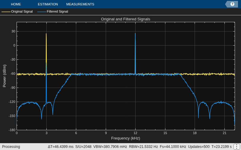
Filter a noisy input signal with the fourth-order section filter. Visualize the spectra of the original signal and the filtered signal using the spectrum analyzer.
The input is a sum of two sine waves with frequencies 3 kHz and 12 kHz, respectively. The input sample rate is 44.1 kHz, and the frame size is set to 1024 samples.
fs = 44100;
FrameLength = 1024;

SINE1 = dsp.SineWave(SamplesPerFrame=FrameLength,SampleRate=fs,Frequency=3000);
SINE2 = dsp.SineWave(SamplesPerFrame=FrameLength,SampleRate=fs,Frequency=12000);
Initialize a spectrum analyzer to visualize the signal spectra.
scope = spectrumAnalyzer(...
    SampleRate=fs,...
    PlotAsTwoSidedSpectrum=false,...
    Title="Original and Filtered Signals",...
    ShowLegend=true,...
    YLimits=[-180 50],...
    ChannelNames={"Original Signal","Filtered Signal"});
for index = 1:1000
    x = SINE1() + SINE2()+ 0.001*randn(FrameLength,1);
    y = fos(x);
    scope([x,y]);
end
Since R2026b
Define the numerator and denominator coefficients for a bandpass fourth-order section filter.
num = [1.0223   -1.9368    0.9205         0         0
    1.5171    2.3980    1.4317    0.6416    0.2752];

den = [1.0000    -1.9368    0.9428         0         0
    1.0000    2.0136    1.9224    1.0260    0.3016];
Create the dsp.FourthOrderSectionFilter object with fixed-point properties. Specify the rounding method, overflow action, and data types for filter coefficients, accumulator, and filter output.
fos = dsp.FourthOrderSectionFilter(num,den,...
    RoundingMethod="Floor",...
    OverflowAction="Wrap",...
    CoefficientsDataType=numerictype(1,16,14),...
    AccumulatorDataType=numerictype(1,32,20),...
    OutputDataType=numerictype(1,16,14))
fos =
  FourthOrderSectionFilter with properties:

               Numerator: [2×5 double]
             Denominator: [2×5 double]
          RoundingMethod: 'Floor'
          OverflowAction: 'Wrap'
    CoefficientsDataType: [1×1 embedded.numerictype]
     AccumulatorDataType: [1×1 embedded.numerictype]
          OutputDataType: [1×1 embedded.numerictype]
Generate a sinusoidal input signal using the dsp.SineWave object with a frequency of 100 Hz and a sample rate of 1000 Hz. Convert the signal to signed fixed-point with a word length of 16 bits and a fraction length of 14 bits.
fs = 1000;
frameSize = 256;
sineGen = dsp.SineWave(Frequency=100,SampleRate=fs,...
    SamplesPerFrame=frameSize);
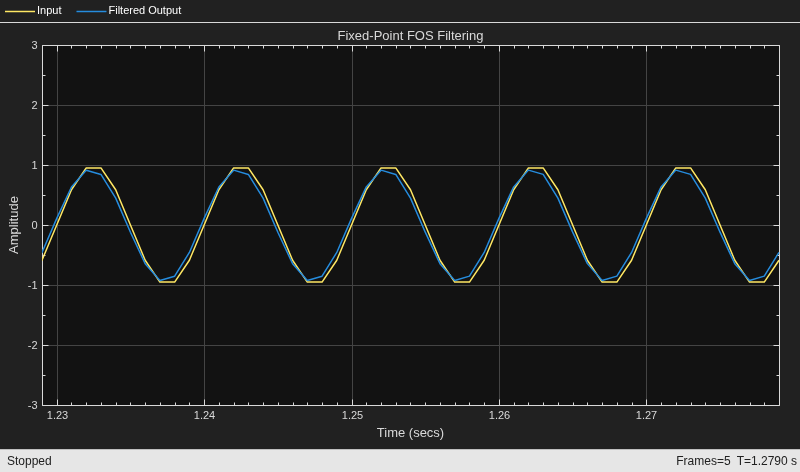
Create a timescope object to visualize the input and filtered output signals.
scope = timescope(SampleRate=fs,...
    TimeSpanSource="property",...
    TimeSpan=0.05,...
    ShowLegend=true,...
    YLimits = [-3 3],...
    ChannelNames={"Input","Filtered Output"},...
    Title="Fixed-Point FOS Filtering");
Generate the sine wave, convert to fixed point, and filter through the FOS filter. Visualize the input and output signals using the time scope.
for i = 1:5
    x = fi(sineGen(),1,16,14);
    y = fos(x);
    scope([x,y]);
end
release(scope);
Since R2026b
Define the numerator and denominator coefficients for a bandpass fourth-order section filter.
num = [1.0223   -1.9368    0.9205         0         0
    1.5171    2.3980    1.4317    0.6416    0.2752];

den = [1.0000    -1.9368    0.9428         0         0
    1.0000    2.0136    1.9224    1.0260    0.3016];
Create two dsp.FourthOrderSectionFilter objects — one for floating-point processing and one for fixed-point processing.
fosFlt = dsp.FourthOrderSectionFilter(num,den);

fosFix = dsp.FourthOrderSectionFilter(num,den,...
    RoundingMethod="Floor",...
    OverflowAction="Wrap",...
    CoefficientsDataType=numerictype(1,16,14));
Generate a sinusoidal input signal using the dsp.SineWave object with a frequency of 100 Hz and a sample rate of 1000 Hz.
fs = 1000;
frameSize = 256;
sineGen = dsp.SineWave(Frequency=100,SampleRate=fs,...
    SamplesPerFrame=frameSize);
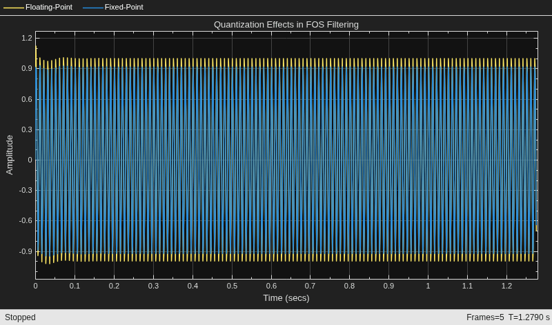
Create a timescope object to visualize the floating-point and fixed-point filter outputs.
scope = timescope(SampleRate=fs,...
    TimeSpanSource="property",...
    TimeSpan=0.05,...
    ShowLegend=true,...
    ChannelNames={"Floating-Point","Fixed-Point"},...
    Title="Quantization Effects in FOS Filtering");
Generate the sinusoidal signal. Pass the signal through both the floating-point FOS filter and the fixed-point FOS filter. Visualize the filtered outputs using the time scope and compare them to observe the quantization effects.
for i = 1:5
    xDouble = sineGen();
    xFixed = fi(xDouble,1,16,14);
    yFlt = fosFlt(xDouble);
    yFix = fosFix(xFixed);
    scope([yFlt,yFix]);
end
release(scope);
Compute the maximum absolute error between the floating-point and fixed-point outputs from the last frame.
maxError = max(abs(yFlt - double(yFix)))
maxError =
0.0842
Since R2026a
Specify the input sample rate explicitly while constructing the dsp.FourthOrderSectionFilter object using the SampleRate argument.
fosFilt = dsp.FourthOrderSectionFilter(SampleRate=22050)
fosFilt =
  FourthOrderSectionFilter with properties:

               Numerator: [1 0.1000 0.2000 0.3000 0.4000]
             Denominator: [1 0.1000 0.2000 0.3000 0.4000]
          RoundingMethod: 'Floor'
          OverflowAction: 'Wrap'
    CoefficientsDataType: [1×1 embedded.numerictype]
     AccumulatorDataType: 'Inherit: Inherit via internal rule'
          OutputDataType: 'Inherit: Same as input'
You can view this information using the Input sample rate field of the info function.
info(fosFilt)
ans = 7×31 char array
    'Discrete-Time IIR Filter (real)'
    '-------------------------------'
    'Filter Structure  : Cascade    '
    'Number of Stages  : 1          '
    'Stable            : Yes        '
    'Linear Phase      : No         '
    'Input sample rate : 22050      '
To specify the input sample rate after constructing the object, use the setInputSampleRate function.
setInputSampleRate(fosFilt,44100)
To confirm, view the sample rate information using the info function.
info(fosFilt)
ans = 7×31 char array
    'Discrete-Time IIR Filter (real)'
    '-------------------------------'
    'Filter Structure  : Cascade    '
    'Number of Stages  : 1          '
    'Stable            : Yes        '
    'Linear Phase      : No         '
    'Input sample rate : 44100      '

