Represent Univariate Dynamic Conditional Mean Models in MATLAB
This topic gives an overview on how to represent a univariate, dynamic, linear conditional mean model, such as an autoregressive, integrated, moving
average (ARIMA) model, in MATLAB® by using the Econometrics Toolbox™
arima object framework. Specifically, the topic shows how to create
nonseasonal and seasonal ARIMA models by using programmatic and interactive workflows;
the former workflow uses the arima function and the latter workflow uses
the Econometric
Modeler app.
Before creating an ARIMA model for time series data, you must determine a model or set of models for your data. For details, see Programmatically Select ARIMA Model for Time Series Using Box-Jenkins Methodology.
Model Creation Overview
You create a univariate, dynamic, linear conditional mean model for a response
series yt at the command line by using the
arima function. The
arima function creates an arima model object, which is a variable that encapsulates the
functional form of the conditional mean model of interest. An arima
object created this way exists independently of data, in other words, you do not
need to fit a model to data to create one. In contrast, the Econometric
Modeler requires that you fit a model to data when you create one.
Regardless of how you create an arima object, it has these characteristics:
It stores your specifications of the model, such as the model structure and parameter values, in properties of the object.
It facilitates model operations, for example, at the command line, you can pass an
arimaobject, specifying the model structure and containing unknown parameters, and data to theestimatefunction to estimate the unknown parameters.
To illustrate the contents of an arima object, create a default
ARIMA model by calling arima without inputs.
Mdl = arima
Mdl =

  arima with properties:

     Description: "ARIMA(0,0,0) Model (Gaussian Distribution)"
      SeriesName: "Y"
    Distribution: Name = "Gaussian"
               P: 0
               D: 0
               Q: 0
        Constant: NaN
              AR: {}
             SAR: {}
              MA: {}
             SMA: {}
     Seasonality: 0
            Beta: [1×0]
        Variance: NaN
MATLAB returns a standard object display, with properties listed to the left
and their corresponding values to the right. By default, arima
sets, to 0, required structural properties, which correspond to
the degrees of the lag operator polynomials in the model. It
sets the sole coefficient and model variance to NaN. The default
ARIMA model has no dynamic responses (lag operator polynomials have degree 0); it is
a simple mean model yt =
c + εt, where the
values of c (Constant property) and the
variance of the innovations (Variance property) are in the
model but their values are unknown.
The default arima object is simplistic; you can create richer
ARIMA models by using one of these two syntaxes or Econometric Modeler (see Specify Model Using Econometric Modeler App):
arima(—This shorthand syntax quickly creates a nonseasonal ARIMA(p,D,q)p,D,q) model, prepared for estimation, with a degreepnonseasonal AR lag polynomial,Ddegrees of nonseasonal integration, and a degreeqnonseasonal MA lag polynomial. For example,arima(4,0,1)creates an ARMA(4,1) model containing unknown coefficients and innovations variance. For more details, see Create ARIMA(p,D,q) Model Using Shorthand Syntax.arima(Property1=Value1,Property2=Value2,...)—This longhand syntax enables you to create more complex models, such as seasonal ARIMA models (SARIMA), and specify values for parameters, by using name-value argument syntax. For example,arima(ARLags=1:4,MALags=1)also creates an ARMA(4,1) model containing unknown coefficients and innovations variance. For more details, see Create ARIMA(p,D,q) Model Using Longhand Syntax and Create Seasonal ARIMA (SARIMA) Models Using Name-Value Arguments.
ARIMA Model Parameters and Corresponding Object Properties
Regardless of how you plan to create a model, observe that model parameters correspond to object properties. Therefore, before you represent a model in MATLAB, it is integral to understand the model equations, their formats, and their parameters. This table contains the general equations of a univariate, dynamic, linear conditional mean model, in lag operator polynomial and difference-equation notation. In the equations, yt is the response series, xt is a collection of exogenous series, and εt is a random series of innovations.
| Notation | Equation |
|---|---|
| Lag operator polynomial | The general equation is The compound autoregressive polynomial a(L) and the compound moving average (MA) polynomial b(L) are often expressed in their expanded form, as polynomial factors for nonseasonal and seasonal effects and integration: Refer to this equation when building a model in MATLAB. |
| Difference equation |
This equation results from expanding the lag operator polynomial equation, and then solving for yt. The equation demonstrates the dynamic nature of the system more clearly than the lag operator polynomial equation. |
Model parameters have these characteristics:
Most model parameters map exactly to object properties, for example,
arimastores the autoregressive (AR) coefficient of an AR(1) model in theARproperty and it stores the degree of nonseasonal integration D in theDproperty.Parameters are non-estimable or estimable:
Non-estimable parameters cannot be fit to data; they typically control the structure of the model. Although the software sets default values to the corresponding properties in some cases, typically, you should set them appropriately for your problem, either explicitly or indirectly such that the software can infer the appropriate values. For example, in the default model,
arimaset propertiesP,D, andQto0; the corresponding parameters are not estimable.Estimable parameters, which include model coefficients and the innovations variance, can be fit to data. Parameters configured for estimation have corresponding property values set to
NaN. For example, in the default model,arimasetsConstantandVariancetoNaN; this setting prepares the corresponding parameters, c and σ2, respectively, for estimation.
This table describes the model parameters and corresponding properties.
| Model Component/Parameter | Description | arima Property | Estimable? |
|---|---|---|---|
a p-degree stable nonseasonal AR polynomial. |
| {ϕ1,ϕ2,…,ϕp} are estimable. | |
| p | Nonseasonal AR polynomial degree | p does not map to a property, but it
contributes to P (see notes below). You can
specify p using shorthand syntax or
arima infers it from other specifications
(ARLags or
AR). | No |
| D | Degree of nonseasonal integration | D | No |
, a ps-degree stable, multiplicative seasonal AR polynomial. |
| {Φp1,Φp2,…,Φps} are estimable. | |
| ps | Seasonal AR polynomial degree | ps does not map to a
property, but it contributes to P (see notes
below). arima infers
ps from other
specifications (SARLags or
SAR). | No |
| s | Seasonality, or the degree of the seasonal differencing polynomial |
| No |
| Ds | Degree of seasonal integration | No corresponding property, but:
| Not applicable |
| c | Model constant | Constant | Yes |
| β | Regression coefficient of exogenous covariates | Beta | Yes |
a q-degree invertible nonseasonal MA polynomial. | MA stores the coefficients
{θ1,θ2,…,θq};
indices correspond to lag exponents, which are customizable by
setting the MALags name-value
argument.. | {θ1,θ2,…,θq} are estimable. | |
| q | Nonseasonal MA polynomial degree | q does not map to a property, but it
contributes to Q (see notes below). You can
specify q using shorthand syntax or
arima infers it from other specifications
(MALags or
MA). | No |
, a qs-degree invertible, multiplicative seasonal MA polynomial. | SMA stores the coefficients
{Θq1,Θq2,…,Θqs};
indices correspond to lag exponents, which are customizable by
setting the SMALags name-value
argument.. | {Θq1,Θq2,…,Θqs} are estimable. | |
| qs | Seasonal MA polynomial degree | qs does not map to a
property, but it contributes to Q (see notes
below). arima infers
qs from other
specifications (SMALags or
SMA). | No |
| εt | Series of random iid Gaussian or Student's t innovations, with mean 0 and variance σ2 | Distribution stores the distribution name
and any distribution-specific parameters (e.g., degrees of freedom
ν). Variance stores the
value of σ2. | σ2 is estimable. The distribution is not estimable, but ν is estimable when the distribution is Student's t. |
Each of the model parameters p, q,
ps, and
qs does not have a one-to-one
mapping to a property. arima combines the polynomial degree
parameters and stores them in properties as follows:
The model property
P= p + D + ps + s; it is the degree w of the compound AR polynomial a(L).Pspecifies the lag of past (presample) observations required to initialize the model.The model property
Q= q + qs; it is the degree v of the compound MA polynomial b(L).Qspecifies the lag of past innovations or conditional variances required to initialize the model.
Model Creation for Calibration Versus Estimation
Programmatic workflows that use the arima function are
flexible because they give you full control over the model structure and parameter
values. Specifically, you can create the following types of models:
Fully specified model — You assign numeric values to all parameters, regardless of whether they are estimable, by using name-value argument syntax when you call
arimaor dot notation after you create a model. A fully specified model is useful when you want to calibrate an entire model, that is, fix all parameters at specific values. You can execute any operation on fully specified models except for estimation (for example, forecast responses from a calibrated model by passing the model to theforecastfunction).Partially specified model — At least one estimable parameter is unknown and you plan to fit the model to data. You can think of a partially specified model as a template for estimation;
NaN-valued parameters indicate to theestimatefunction which parameters to fit to data (estimateaccepts a partially specified model and data, and then returns a fully specified model). The only operation you can perform on a partially specified model is estimation.
Interactive workflows in Econometric Modeler create only partially specified models for estimation. The app directs you through model creation by using dialogs for model types, for example

To illustrate the differences between partially and fully specified models, at the command line, create the partially specified AR(1) model yt = 1 + ϕyt–1 + εt.
Mdl = arima(Constant=1,ARLags=1) % Partially specified model
Mdl =

  arima with properties:

     Description: "ARIMA(1,0,0) Model (Gaussian Distribution)"
      SeriesName: "Y"
    Distribution: Name = "Gaussian"
               P: 1
               D: 0
               Q: 0
        Constant: 1
              AR: {NaN} at lag [1]
             SAR: {}
              MA: {}
             SMA: {}
     Seasonality: 0
            Beta: [1×0]
        Variance: NaN
Because AR contains a NaN and
Variance is NaN, the corresponding
parameters ϕ and σ2
are unknown and estimable.
Set the unknown parameters ϕ to 0.5 and
σ2 to 0.25 by using dot notation.
Specify the AR property as a cell vector
of numeric scalars; each cell corresponds to an AR coefficient in the model.
Mdl.AR = {0.5};
Mdl.Variance = 0.25
Mdl =
arima with properties:
Description: "ARIMA(1,0,0) Model (Gaussian Distribution)"
SeriesName: "Y"
Distribution: Name = "Gaussian"
P: 1
D: 0
Q: 0
Constant: 1
AR: {0.5} at lag [1]
SAR: {}
MA: {}
SMA: {}
Seasonality: 0
Beta: [1×0]
Variance: 0.25No properties contain NaN values. Therefore,
Mdl is fully specified.
Create ARIMA(p,D,q) Model Using Shorthand Syntax
The ARIMA(p,D,q) model is a nonseasonal model of the form:
At the command line, you can specify a model of this form using the shorthand
syntax
arima(.
For the input arguments p,D,q)pDq
When you use this shorthand syntax, arima creates an
arima model with these default settings.
| Property Name | Value | Description |
|---|---|---|
P | Sum of the input numeric scalars p and D | The number of presample responses required to initialize the model (the order of the nonseasonal AR polynomial p plus the level of nonseasonal integration D) |
D | Input numeric scalar D | Degree of nonseasonal integration, D |
Q | Input numeric scalar q | The number of presample innovations required to initialize the model (the order of nonseasonal MA polynomial q) |
Constant | NaN | Model constant c is present and estimable |
AR | Length p cell vector of
NaNs | All nonseasonal AR coefficients ϕj, j = 1 through p, are present and estimable |
SAR | Empty cell vector {} | Seasonal AR polynomial Φ(L) is not present |
MA | Length q cell vector of
NaNs | All MA coefficients θk, k = 1 through q, are present and estimable |
SMA | Empty cell vector {} | Seasonal MA polynomial Θ(L) is not present |
Seasonality | 0 | No seasonal integration s |
Beta | Empty vector [] | No exogenous regression component xt′β is present in the model |
Distribution | "Gaussian" | Innovations εt are Gaussian |
Variance | NaN | Model variance σ2 is present and estimable |
For nonseasonal models, the inputs Dqarima assigns to properties D and
Q. However, the input argument
parima assigns to the model property P.
P stores the number of presample observations needed to
initialize the AR component of the model. The required number of presample
observations is p + D.
Consider specifying the ARIMA(2,1,1) model
where the innovation process is Gaussian with (unknown) constant variance.
Mdl = arima(2,1,1)
Mdl =

  arima with properties:

     Description: "ARIMA(2,1,1) Model (Gaussian Distribution)"
    Distribution: Name = "Gaussian"
               P: 3
               D: 1
               Q: 1
        Constant: NaN
              AR: {NaN NaN} at lags [1 2]
             SAR: {}
              MA: {NaN} at lag [1]
             SMA: {}
     Seasonality: 0
            Beta: [1×0]
        Variance: NaN
The model property P does not have value 2 (the AR degree).
With the integration, a total of p + D (here,
2 + 1 = 3) presample observations are needed to initialize the AR component of the
model.
The partially specified model Mdl has NaNs
for all estimable parameters (coefficients and innovations variance). A
NaN value is a placeholder signaling that the corresponding
parameter is prepared for estimation.
To set different values for any properties, you can modify the created model
object using dot notation. For example, set the variance of Mdl
to 0.5.
Mdl.Variance = 0.5
Mdl =

  arima with properties:

     Description: "ARIMA(2,1,1) Model (Gaussian Distribution)"
      SeriesName: "Y"
    Distribution: Name = "Gaussian"
               P: 3
               D: 1
               Q: 1
        Constant: NaN
              AR: {NaN NaN} at lags [1 2]
             SAR: {}
              MA: {NaN} at lag [1]
             SMA: {}
     Seasonality: 0
            Beta: [1×0]
        Variance: 0.5
To estimate parameters, pass the model and data to estimate. This returns a fitted, fully specified
arima object with the same structure as the input model. The
fitted model contains parameter estimates for each NaN valued
property.
Create ARIMA(p,D,q) Model Using Longhand Syntax
The most flexible way to create a conditional mean model is by using the longhand
syntax, or, setting property values using name-value arguments. You do not need, nor
are you able, to specify a value for every model object property.
arima assigns default values to any properties you do not (or
cannot) specify.
In condensed, lag operator notation, nonseasonal ARIMA(p,D,q) models are of the form
| (1) |
The innovations εt can take one of the
following forms, which you set using the Distribution name-value
argument:
Independent and identically distributed Gaussian distribution with mean 0 and constant variance σ2 (the default)
Independent and identically distributed central Student’s t with ν degrees of freedom
Dependent Gaussian or Student’s t with a conditional variance process σt2 (for example, a GARCH model). Specify the conditional variance model specifying a
garch,egarch, orgjrmodel.
You can specify the following name-value arguments to create nonseasonal
arima models.
Name-Value Arguments for Nonseasonal ARIMA Models
| Name | Corresponding Model Term(s) in Equation 1 | When to Specify |
|---|---|---|
AR | Nonseasonal AR coefficients, | Calibrate, or specify equality constraints during estimation for, the AR coefficients. For example, to specify the AR coefficients in the model specify You need only specify the
nonzero elements of Any coefficients you specify must correspond to a stable AR operator polynomial. |
ARLags | Lags corresponding to nonzero, nonseasonal AR coefficients |
Use this argument to customize the nonzero lags
of the Set |
Beta | Values of the coefficients of the exogenous covariates | Calibrate, or specify equality constraints during
estimation for, the exogenous regression coefficients. For
example, use By default,
|
Constant | Constant term, c | Calibrate, or specify equality constraints during estimation
for, the model constant. For example, for a model with no
constant term, specify
Constant=0.By default, Constant has value
NaN. |
D | Degree of nonseasonal differencing, D | Specify a degree of nonseasonal differencing greater than
zero. For example, to specify one degree of differencing,
specify D=1.By default, D has value 0 (meaning
no nonseasonal integration). |
Distribution | Distribution of the innovation process | Specify a Student’s t innovation
distribution. By default, the innovation distribution is
Gaussian. For example, to specify a t distribution with unknown degrees of freedom, specify Distribution="t".To specify a t innovation distribution with known degrees of freedom, assign Distribution a
structure array with fields Name and
DoF. For example, for a
t distribution with nine degrees of
freedom, specify
Distribution=struct("Name","t","DoF",9). |
MA | Nonseasonal MA coefficients, | Calibrate, or specify equality constraints during estimation for, the MA coefficients. For example, to specify the MA coefficients in the model specify You need only specify the
nonzero elements of Any coefficients you specify must correspond to an invertible MA polynomial. |
MALags | Lags corresponding to nonzero, nonseasonal MA coefficients |
Use this argument to customize the
nonzero lags of the specify Set |
Variance |
|
|
This table contains examples of nonseasonal models and how to specify them by
using arima.
| Model | Specification |
|---|---|
AR(1), all coefficients are unknown
|
|
ARMA(8,4), all coefficients are known
| arima(ARLags=[4 8],MALags=4) |
MA(2), all coefficients are unknown
| arima(Constant=0,MA={NaN
NaN},Distribution="t") or
arima(Constant=0,MALags=[1
2],Distribution="t") |
Fully specified ARIMA(1,1,1)
| arima(Constant=0.2,AR={0.8},MA={0.6},D=1,Variance=0.1^2,
... |
Create Seasonal ARIMA (SARIMA) Models Using Name-Value Arguments
For a time series with periodicity s, ps is the degree of the seasonal AR lag operator polynomial and qs is the degree of the seasonal MA lag operator polynomial . A multiplicative seasonal ARIMA model (SARIMA) with degree D nonseasonal integration, degree s seasonality, and one degree of seasonal integration, is
| (2) |
In addition to the arguments for specifying nonseasonal models (described in Name-Value Arguments for Nonseasonal ARIMA Models), you can specify these name-value arguments to create a SARIMA model.
Name-Value Arguments for Seasonal ARIMA Models
| Argument | Corresponding Model Term(s) in Equation 2 | When to Specify |
|---|---|---|
SAR | Seasonal AR coefficients, | Calibrate, or specify equality constraints during estimation for, the seasonal AR coefficients. When specifying AR coefficients, use the sign opposite to what appears in Equation 2 (that is, use the sign of the coefficient as it would appear on the right side of the equation). Use
For example, to specify the model specify
Any coefficient values you enter must correspond to a stable seasonal AR polynomial. |
SARLags | Lags corresponding to nonzero seasonal AR coefficients, in the periodicity of the observed series |
Use this argument to customize the
nonzero lags of the For example, to specify the model specify
|
SMA | Seasonal MA coefficients, | Calibrate, or specify equality constraints during estimation for, the seasonal MA coefficients. Use For example, to specify the model specify
Any coefficient values you enter must correspond to an invertible seasonal MA polynomial. |
SMALags | Lags corresponding to the nonzero seasonal MA coefficients, in the periodicity of the observed series |
Use this argument to customize the
nonzero lags of the For example, to specify the model specify
|
Seasonality | Seasonal periodicity, s | Specify the degree of seasonal integration
s in the seasonal differencing polynomial
Δs = 1 –
Ls. For
example, to specify the periodicity for seasonal integration of
monthly data, specify
Seasonality=12.If you specify nonzero Seasonality, then the degree
of the whole seasonal differencing polynomial is one. By
default, Seasonality has value
0 (meaning periodicity and no seasonal
integration). |
This table contains examples of seasonal models and how to specify them by using
arima.
| Model | Specification |
|---|---|
|
|
| arima(ARLags=[4 8],MALags=4) |
| arima(Constant=0,MA={NaN
NaN},Distribution="t") or
arima(Constant=0,MALags=[1
2],Distribution="t") |
| arima(Constant=0.2,AR={0.8},MA={0.6},D=1,Variance=0.1^2,
... |
Create Conditional Mean Model Containing Exogenous Linear Regression Term
You can include an exogenous linear regression term in any univariate conditional mean model. For simplicity, consider including an exogenous linear regression terms in an ARIMA model. The result is an ARIMAX(p,D,q) model and it has the form
| (3) |
In addition to the properties associated with nonseasonal and
seasonal
parameters, ARIMAX models contain the property Beta.
Name-Value Arguments for ARIMAX Models
| Argument | Corresponding Model Term(s) in Equation 2 | When to Specify |
|---|---|---|
Beta | Exogenous linear regression coefficient, β | Calibrate, or specify equality constraints during
estimation for, β. For example, use
By default,
|
The following conditions apply to models with an exogenous regression component:
Econometrics Toolbox model objects are agnostic of data; models are aware of all associated series, response and exogenous predictors, after you create a model and when you operate on it using functions that require input data.
If you plan to estimate β, do not specify
Betawhen you callarima.arimainfers the number of regression coefficients from the number of variables in the input exogenous predictor data.If you specify a nonzero
D, the software differences the response series yt before the predictors enter the model. You should preprocess the exogenous covariates xt by testing for stationarity and differencing if any are unit root nonstationary.If any nonstationary exogenous predictor enters the model, the false negative rate for significance tests of β can increase.
This table contains examples of models containing an exogenous regression component.
| Model | Specification |
|---|---|
ARX(1), all coefficients are unknown, one exogenous predictor xt
| All the following lines specify this model:
|
Fully specified ARIMAX(1,1,1), 2 exogenous predictors x1,t and x2,t
| arima(Constant=0.2,AR={0.8},MA={0.6},D=1,Variance=0.1^2,
... |
Specify Model Using Econometric Modeler App
You can specify the lag structure and innovation distribution of seasonal and nonseasonal conditional mean models using the Econometric Modeler app. The app treats all coefficients as unknown and estimable, including the degrees of freedom parameter for a t innovation distribution. Econometric Modeler
At the command line, open the Econometric Modeler app.
econometricModeler
Alternatively, open the app from the apps gallery (see Econometric Modeler).
In the app, you can see all supported models by selecting a time series variable for the response in the Time Series pane. Then, on the Modeler tab, in the Models section, click the arrow to display the models gallery.
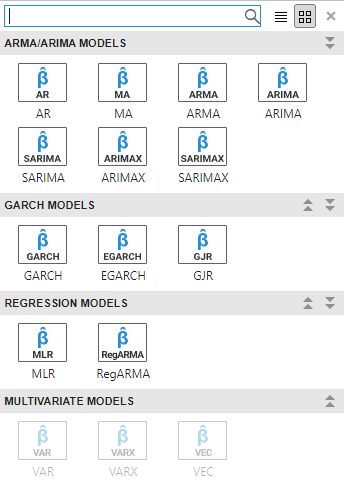
The ARIMA Models section contains supported conditional mean models.
For conditional mean model estimation, SARIMA and SARIMAX are the most flexible models. You can create any conditional mean model that excludes exogenous predictors by clicking SARIMA, or you can create any conditional mean model that includes at least one exogenous predictor by clicking SARIMAX.
After you select a model, the app displays the Type Model
Parameters dialog box, where Type is the model
type. This figure shows the SARIMAX Model Parameters dialog box.
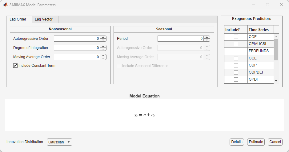
Adjustable parameters in the dialog box depend on Type.
In general, adjustable parameters include:
A model constant and linear regression coefficients corresponding to predictor variables
Time series component parameters, which include seasonal and nonseasonal lags and degrees of integration
The innovation distribution
As you adjust parameter values, the equation in the Model
Equation section changes to match your specifications. Adjustable
parameters correspond to input and name-value arguments as described in Create ARIMA(p,D,q) Model Using Longhand Syntax,
Create Seasonal ARIMA (SARIMA) Models Using Name-Value Arguments, and arima.
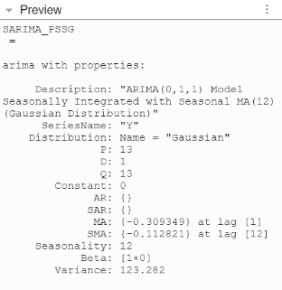
Econometric Modeler always creates estimated models. After you specify
the model structure, select Estimate to fit the model. You
can inspect the resulting arima model in the Preview pane, for
example
For more details on specifying models using the app, see Fit Models to Data and Specifying Univariate Lag Operator Polynomials Interactively.
What Are Conditional Mean Models?
Consider the univariate random variable yt. The unconditional mean of yt is the expected value of yt, E(yt). In contrast, the conditional mean of yt is the expected value of yt given a conditioning set of variables, Ωt.
A conditional mean model specifies a functional form for E(yt| Ωt).
For a static conditional mean model, the conditioning set of variables is measured contemporaneously with the dependent variable yt. An example of a static conditional mean model is the ordinary linear regression model. Suppose the conditioning set Ωt = xt, a row vector of exogenous covariates measured at time t, and β, a column vector of coefficients. The conditional mean of yt is the linear combination
In time series econometrics, often the dynamic behavior of a variable over time is of interest. A dynamic conditional mean model is a stochastic process that specifies the expected value of yt as a function of historical information. Let Ωt = Ht–1 denote the history of the process available at time t. A dynamic conditional mean model specifies the evolution of the conditional mean, E(yt| Ht–1). Examples of historical information are:
Past observations, y1, y2,...,yt–1
Vectors of past exogenous variables, x1,x2,…,xt–1.
Past innovations, ε1,ε2,…,εt–1.
Stationary processes play an important role in time series analysis. A stochastic process is covariance stationary when its expected value, variance, and covariance between elements of the series are independent of time.
For example, the MA(q) model, with c = 0, is stationary for any nonnegative integer q < ∞ because each of the following are free of t for all time points [1].
A time series is a unit root process when its expected value, variance, or covariance grows with time. Consequently, the time series is nonstationary.
The constant mean property of stationarity does not preclude the possibility of a dynamic conditional expectation process. The serial autocorrelation between lagged observations exhibited by many time series suggests the expected value of yt depends on historical information. By Wold’s decomposition [2], the conditional mean of any stationary process yt is
| (4) |
Any model of the general linear form given by Equation 4 is a valid specification for the dynamic behavior of a stationary stochastic process. Special cases of stationary stochastic processes are the autoregressive (AR) model, moving average (MA) model, and the autoregressive moving average (ARMA) model.
References
[1] Box, George E. P., Gwilym M. Jenkins, and Gregory C. Reinsel. Time Series Analysis: Forecasting and Control. 3rd ed. Englewood Cliffs, NJ: Prentice Hall, 1994.
[2] Wold, Herman. "A Study in the Analysis of Stationary Time Series." Journal of the Institute of Actuaries 70 (March 1939): 113–115. https://doi.org/10.1017/S0020268100011574.
See Also
Apps
Objects
Functions
Topics
- Create Autoregressive (AR) Models
- Create Moving Average (MA) Models
- Create Autoregressive Moving Average (ARMA) Models
- Create Autoregressive Integrated Moving Average (ARIMA) Models
- Create ARIMA Models That Include Exogenous Covariates
- Create Seasonal ARIMA (SARIMA) Models
- Modify Properties of Conditional Mean Model Objects
- Specify Conditional Mean Model Innovation Distribution
- Model Seasonal Lag Effects Using Indicator Variables