Plotting Sensitivities of a Portfolio of Options
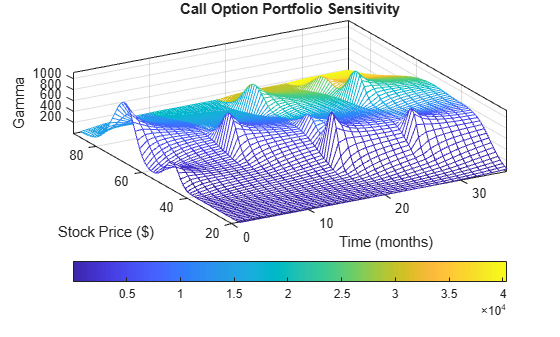
This example plots gamma as a function of price and time for a portfolio of ten Black-Scholes options.
The plot in this example shows a three-dimensional surface. For each point on the surface, the height (z-value) represents the sum of the gammas for each option in the portfolio weighted by the amount of each option. The x-axis represents changing price, and the y-axis represents time. The plot adds a fourth dimension by showing delta as surface color. This example has applications in hedging. First set up the portfolio with arbitrary data. Current prices range from $20 to $90 for each option. Then, set the corresponding exercise prices for each option.
Range = 20:90;
PLen = length(Range);
ExPrice = [75 70 50 55 75 50 40 75 60 35];
Set all risk-free interest rates to 10%, and set times to maturity in days. Set all volatilities to 0.35. Set the number of options of each instrument, and allocate space for matrices.
Rate = 0.1*ones(10,1);
Time = [36  36  36  27  18  18  18  9  9  9];
Sigma = 0.35*ones(10,1);
NumOpt = 1000*[4  8  3  5  5.5  2  4.8  3  4.8  2.5];
ZVal = zeros(36, PLen);
Color = zeros(36, PLen);
For each instrument, create a matrix (of size Time by PLen) of prices for each period.
for i = 1:10
    Pad = ones(Time(i),PLen);
    NewR = Range(ones(Time(i),1),:);
Create a vector of time periods 1 to Time and a matrix of times, one column for each price.
  T = (1:Time(i))';
  NewT = T(:,ones(PLen,1));
Use the Black-Scholes gamma and delta sensitivity functions blsgamma and blsdelta to compute gamma and delta.
    ZVal(36-Time(i)+1:36,:) = ZVal(36-Time(i)+1:36,:) ...
        + NumOpt(i) * blsgamma(NewR, ExPrice(i)*Pad, ...
        Rate(i)*Pad, NewT/36, Sigma(i)*Pad);

    Color(36-Time(i)+1:36,:) = Color(36-Time(i)+1:36,:) ...
        + NumOpt(i) * blsdelta(NewR, ExPrice(i)*Pad, ...
        Rate(i)*Pad, NewT/36, Sigma(i)*Pad);
end
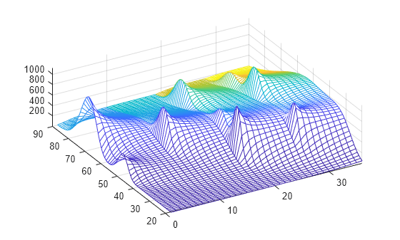
Draw the surface as a mesh, set the viewpoint, and reverse the x-axis because of the viewpoint. The axes range from 20 to 90, 0 to 36, and -∞ to ∞.
mesh(Range, 1:36, ZVal, Color);
view(60,60);
set(gca, 'xdir','reverse', 'tag', 'mesh_axes_3');
axis([20 90  0 36  -inf inf]);
Add a title and axis labels and draw a box around the plot. Annotate the colors with a bar and label the color bar.
title('Call Option Portfolio Sensitivity');
xlabel('Stock Price ($)');
ylabel('Time (months)');
zlabel('Gamma');
set(gca, 'box', 'on');
colorbar('horiz');
See Also
bnddury | bndconvy | bndprice | bndkrdur | blsprice | blsdelta | blsgamma | blsvega | zbtprice | zero2fwd | zero2disc | corr2cov | portopt
Topics
- Plotting Sensitivities of an Option
- Pricing and Analyzing Equity Derivatives
- Greek-Neutral Portfolios of European Stock Options
- Sensitivity of Bond Prices to Interest Rates
- Bond Portfolio for Hedging Duration and Convexity
- Bond Prices and Yield Curve Parallel Shifts
- Bond Prices and Yield Curve Nonparallel Shifts
- Term Structure Analysis and Interest-Rate Swaps