Plotting Sensitivities of an Option
This example creates a three-dimensional plot showing how gamma changes relative to price for a Black-Scholes option.
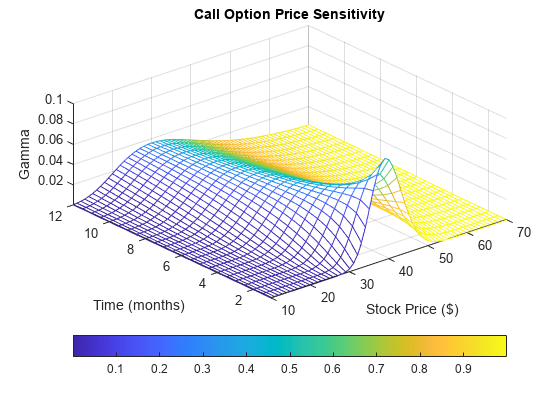
Recall that gamma is the second derivative of the option price relative to the underlying security price. The plot in this example shows a three-dimensional surface whose z-value is the gamma of an option as price (x-axis) and time (y-axis) vary. The plot adds yet a fourth dimension by showing option delta (the first derivative of option price to security price) as the color of the surface. First set the price range of the options, and set the time range to one year divided into half-months and expressed as fractions of a year.
Range = 10:70;
Span = length(Range);
j = 1:0.5:12;
Newj = j(ones(Span,1),:)'/12;
For each time period, create a vector of prices from 10 to 70 and create a matrix of all ones.
JSpan = ones(length(j),1);
NewRange = Range(JSpan,:);
Pad = ones(size(Newj));
Calculate the gamma and delta sensitivities (greeks) using the blsgamma and blsdelta functions. Gamma is the second derivative of the option price with respect to the stock price, and delta is the first derivative of the option price with respect to the stock price. The exercise price is $40, the risk-free interest rate is 10%, and volatility is 0.35 for all prices and periods.
ZVal = blsgamma(NewRange, 40*Pad, 0.1*Pad, Newj, 0.35*Pad);
Color = blsdelta(NewRange, 40*Pad, 0.1*Pad, Newj, 0.35*Pad);
Display the greeks as a function of price and time. Gamma is the z-axis; delta is the color.
mesh(Range, j, ZVal, Color);
xlabel('Stock Price ($)');
ylabel('Time (months)');
zlabel('Gamma');
title('Call Option Price Sensitivity');
axis([10 70  1 12  -inf inf]);
view(-40, 50);
colorbar('horiz');
See Also
bnddury | bndconvy | bndprice | bndkrdur | blsprice | blsdelta | blsgamma | blsvega | zbtprice | zero2fwd | zero2disc | corr2cov | portopt
Topics
- Plotting Sensitivities of a Portfolio of Options
- Pricing and Analyzing Equity Derivatives
- Greek-Neutral Portfolios of European Stock Options
- Sensitivity of Bond Prices to Interest Rates
- Bond Portfolio for Hedging Duration and Convexity
- Bond Prices and Yield Curve Parallel Shifts
- Bond Prices and Yield Curve Nonparallel Shifts
- Term Structure Analysis and Interest-Rate Swaps