histogram
Histogram plot
Description
Histograms are a type of bar plot that group data into bins. After you create
a Histogram object, you can modify aspects of the histogram by
changing its property values. This is particularly useful for quickly modifying the
properties of the bins or changing the display.
Creation
Syntax
Description
Numeric and Time Data
histogram( creates a histogram
plot of X)X. The histogram function uses
an automatic binning algorithm that returns bins with a uniform width,
chosen to cover the range of elements in X and reveal the
underlying shape of the distribution. histogram
displays the bins as rectangular bars such that the height of each rectangle
indicates the number of elements in the bin.
Categorical Data
histogram(
plots only a subset of categories in C,Categories)C.
histogram('Categories',
manually specifies categories and associated bin counts.
Categories,'BinCounts',counts)histogram plots the specified bin counts and does
not do any data binning.
Table Data
histogram(
specifies a subset of categories to use when the table variable has
categorical values. (since R2026a)tbl,datavar,Categories)
Additional Options
histogram(___,
specifies additional parameters using one or more name-value arguments for
any of the previous syntaxes. For example, specify
Name,Value)Normalization to use a different type of
normalization. For a list of properties, see Histogram Properties.
histogram(
plots into the specified axes instead of into the current axes
(ax,___)gca). ax can precede any of the
input argument combinations in the previous syntaxes.
h = histogram(___)Histogram object. Use this to inspect and
adjust the properties of the histogram. For a list of properties, see
Histogram Properties.
Input Arguments
Name-Value Arguments
Specify optional pairs of arguments as
Name1=Value1,...,NameN=ValueN, where Name is
the argument name and Value is the corresponding value.
Name-value arguments must appear after other arguments, but the order of the
pairs does not matter.
Example: histogram(X,BinWidth=5)
Before R2021a, use commas to separate each name and value, and enclose
Name in quotes.
Example: histogram(X,'BinWidth',5)
Note
The properties listed here are only a subset. For a complete list, see Histogram Properties.
Bins
Categories
Data
Color and Styling
Histogram bar color, specified as one of these values:
'none'— Bars are not filled.'auto'— Histogram bar color is chosen automatically (default).RGB triplet, hexadecimal color code, or color name — Bars are filled with the specified color.
RGB triplets and hexadecimal color codes are useful for specifying custom colors.
An RGB triplet is a three-element row vector whose elements specify the intensities of the red, green, and blue components of the color. The intensities must be in the range
[0,1]; for example,[0.4 0.6 0.7].A hexadecimal color code is a character vector or a string scalar that starts with a hash symbol (
#) followed by three or six hexadecimal digits, which can range from0toF. The values are not case sensitive. Thus, the color codes"#FF8800","#ff8800","#F80", and"#f80"are equivalent.
Alternatively, you can specify some common colors by name. This table lists the named color options, the equivalent RGB triplets, and hexadecimal color codes.
Color Name Short Name RGB Triplet Hexadecimal Color Code Appearance "red""r"[1 0 0]"#FF0000"
"green""g"[0 1 0]"#00FF00"
"blue""b"[0 0 1]"#0000FF"
"cyan""c"[0 1 1]"#00FFFF"
"magenta""m"[1 0 1]"#FF00FF"
"yellow""y"[1 1 0]"#FFFF00"
"black""k"[0 0 0]"#000000"
"white""w"[1 1 1]"#FFFFFF"
This table lists the default color palettes for plots in the light and dark themes.
Palette Palette Colors "gem"— Light theme defaultBefore R2025a: Most plots use these colors by default.

"glow"— Dark theme default
You can get the RGB triplets and hexadecimal color codes for these palettes using the
orderedcolorsandrgb2hexfunctions. For example, get the RGB triplets for the"gem"palette and convert them to hexadecimal color codes.RGB = orderedcolors("gem"); H = rgb2hex(RGB);Before R2023b: Get the RGB triplets using
RGB = get(groot,"FactoryAxesColorOrder").Before R2024a: Get the hexadecimal color codes using
H =
            compose("#%02X%02X%02X",round(RGB*255))
.
If you specify DisplayStyle as 'stairs', then
histogram does not use the
FaceColor property.
Example: histogram(X,'FaceColor','g')
Histogram edge color, specified as one of these values:
'none'— Edges are not drawn.'auto'— Color of each edge is chosen automatically.RGB triplet, hexadecimal color code, or color name — Edges use the specified color.
RGB triplets and hexadecimal color codes are useful for specifying custom colors.
An RGB triplet is a three-element row vector whose elements specify the intensities of the red, green, and blue components of the color. The intensities must be in the range
[0,1]; for example,[0.4 0.6 0.7].A hexadecimal color code is a character vector or a string scalar that starts with a hash symbol (
#) followed by three or six hexadecimal digits, which can range from0toF. The values are not case sensitive. Thus, the color codes"#FF8800","#ff8800","#F80", and"#f80"are equivalent.
Alternatively, you can specify some common colors by name. This table lists the named color options, the equivalent RGB triplets, and hexadecimal color codes.
Color Name Short Name RGB Triplet Hexadecimal Color Code Appearance "red""r"[1 0 0]"#FF0000""green""g"[0 1 0]"#00FF00""blue""b"[0 0 1]"#0000FF""cyan""c"[0 1 1]"#00FFFF""magenta""m"[1 0 1]"#FF00FF""yellow""y"[1 1 0]"#FFFF00""black""k"[0 0 0]"#000000""white""w"[1 1 1]"#FFFFFF"This table lists the default color palettes for plots in the light and dark themes.
Palette Palette Colors "gem"— Light theme defaultBefore R2025a: Most plots use these colors by default.
"glow"— Dark theme defaultYou can get the RGB triplets and hexadecimal color codes for these palettes using the
orderedcolorsandrgb2hexfunctions. For example, get the RGB triplets for the"gem"palette and convert them to hexadecimal color codes.RGB = orderedcolors("gem"); H = rgb2hex(RGB);Before R2023b: Get the RGB triplets using
RGB = get(groot,"FactoryAxesColorOrder").Before R2024a: Get the hexadecimal color codes using
H =
            compose("#%02X%02X%02X",round(RGB*255))
.
Example: histogram(X,'EdgeColor','r')
Transparency of histogram bar edges, specified as a scalar value
in the range [0,1]. A value of
1 means fully opaque and 0
means completely transparent (invisible).
Example: histogram(X,'EdgeAlpha',0.5)
Line style, specified as one of the options listed in this table.
| Line Style | Description | Resulting Line |
|---|---|---|
"-" | Solid line |
|
"--" | Dashed line |
|
":" | Dotted line |
|
"-." | Dash-dotted line |
|
"none" | No line | No line |
Output Arguments
Properties
| Histogram Properties | Histogram appearance and behavior |
Examples
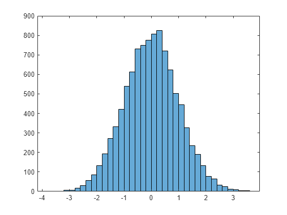
Generate 10,000 random numbers and create a histogram. The histogram function automatically chooses an appropriate number of bins to cover the range of values in x and show the shape of the underlying distribution.
x = randn(10000,1);
h = histogram(x)
h =
  Histogram with properties:

             Data: [10000×1 double]
           Values: [2 2 1 6 7 17 29 57 86 133 193 271 331 421 540 613 730 748 776 806 824 721 623 503 446 326 234 191 132 78 65 33 26 11 8 5 5]
          NumBins: 37
         BinEdges: [-3.8000 -3.6000 -3.4000 -3.2000 -3 -2.8000 -2.6000 -2.4000 -2.2000 -2 -1.8000 -1.6000 -1.4000 -1.2000 -1 -0.8000 -0.6000 -0.4000 -0.2000 0 0.2000 0.4000 0.6000 0.8000 1.0000 1.2000 1.4000 1.6000 1.8000 2.0000 2.2000 … ] (1×38 double)
         BinWidth: 0.2000
        BinLimits: [-3.8000 3.6000]
    Normalization: 'count'
        FaceColor: 'auto'
        EdgeColor: [0.1294 0.1294 0.1294]

  Show all properties
When you specify an output argument to the histogram function, it returns a histogram object. You can use this object to inspect the properties of the histogram, such as the number of bins or the width of the bins.
Find the number of histogram bins.
nbins = h.NumBins
nbins =
37
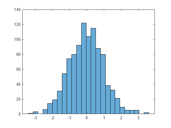
Plot a histogram of 1,000 random numbers sorted into 25 equally spaced bins.
x = randn(1000,1);
nbins = 25;
h = histogram(x,nbins)
h =
  Histogram with properties:

             Data: [1000×1 double]
           Values: [1 3 0 6 14 19 31 54 74 80 92 122 104 115 88 80 38 32 21 9 5 5 5 0 2]
          NumBins: 25
         BinEdges: [-3.4000 -3.1200 -2.8400 -2.5600 -2.2800 -2 -1.7200 -1.4400 -1.1600 -0.8800 -0.6000 -0.3200 -0.0400 0.2400 0.5200 0.8000 1.0800 1.3600 1.6400 1.9200 2.2000 2.4800 2.7600 3.0400 3.3200 3.6000]
         BinWidth: 0.2800
        BinLimits: [-3.4000 3.6000]
    Normalization: 'count'
        FaceColor: 'auto'
        EdgeColor: [0.1294 0.1294 0.1294]

  Show all properties
Find the bin counts.
counts = h.Values
counts = 1×25

     1     3     0     6    14    19    31    54    74    80    92   122   104   115    88    80    38    32    21     9     5     5     5     0     2
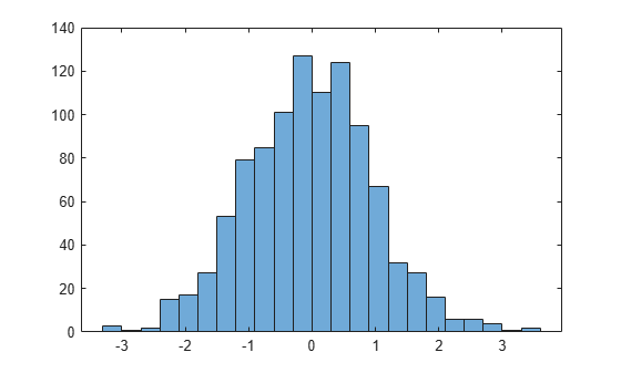
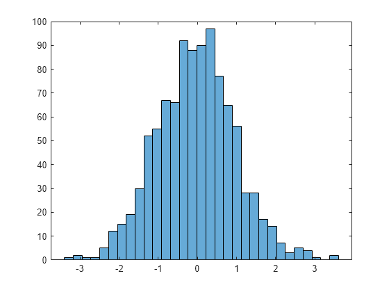
Generate 1,000 random numbers and create a histogram.
X = randn(1000,1);
h = histogram(X)
h =
  Histogram with properties:

             Data: [1000×1 double]
           Values: [3 1 2 15 17 27 53 79 85 101 127 110 124 95 67 32 27 16 6 6 4 1 2]
          NumBins: 23
         BinEdges: [-3.3000 -3.0000 -2.7000 -2.4000 -2.1000 -1.8000 -1.5000 -1.2000 -0.9000 -0.6000 -0.3000 0 0.3000 0.6000 0.9000 1.2000 1.5000 1.8000 2.1000 2.4000 2.7000 3 3.3000 3.6000]
         BinWidth: 0.3000
        BinLimits: [-3.3000 3.6000]
    Normalization: 'count'
        FaceColor: 'auto'
        EdgeColor: [0.1294 0.1294 0.1294]

  Show all properties
Use the morebins function to coarsely adjust the number of bins.
Nbins = morebins(h);
Nbins = morebins(h)
Nbins =
29
Adjust the bins at a fine grain level by explicitly setting the number of bins.
h.NumBins = 31;
Generate 1,000 random numbers and create a histogram. Specify the bin edges as a vector with wide bins on the edges of the histogram to capture the outliers that do not satisfy . The first vector element is the left edge of the first bin, and the last vector element is the right edge of the last bin.
x = randn(1000,1);
edges = [-10 -2:0.25:2 10];
h = histogram(x,edges);
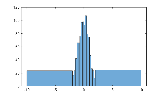
Specify the Normalization property as 'countdensity' to flatten out the bins containing the outliers. Now, the area of each bin (rather than the height) represents the frequency of observations in that interval.
h.Normalization = 'countdensity';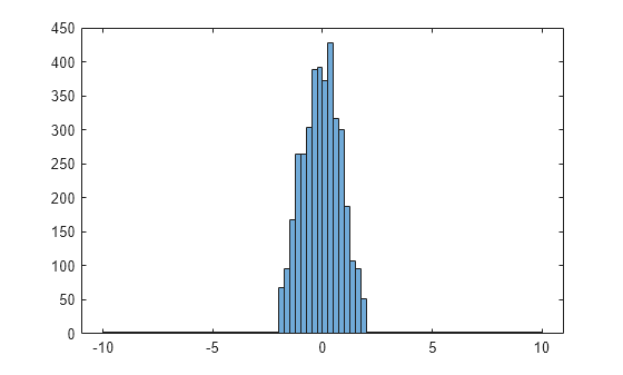
Create a categorical vector that represents votes. The categories in the vector are 'yes', 'no', or 'undecided'.
A = [0 0 1 1 1 0 0 0 0 NaN NaN 1 0 0 0 1 0 1 0 1 0 0 0 1 1 1 1];
C = categorical(A,[1 0 NaN],{'yes','no','undecided'})
C = 1×27 categorical
no no yes yes yes no no no no undecided undecided yes no no no yes no yes no yes no no no yes yes yes yes
Plot a categorical histogram of the votes, using a relative bar width of 0.5.
h = histogram(C,'BarWidth',0.5)
h =
  Histogram with properties:

              Data: [no    no    yes    yes    yes    no    no    no    no    undecided    undecided    yes    no    no    no    yes    no    yes    no    yes    no    no    no    yes    yes    yes    yes]
            Values: [11 14 2]
    NumDisplayBins: 3
        Categories: {'yes'  'no'  'undecided'}
      DisplayOrder: 'data'
     Normalization: 'count'
      DisplayStyle: 'bar'
         FaceColor: 'auto'
         EdgeColor: [0.1294 0.1294 0.1294]

  Show all properties
Since R2026a
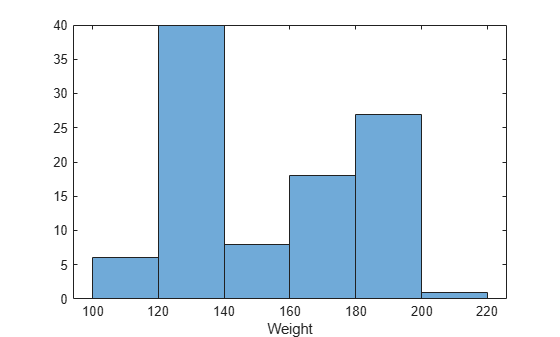
Read patients.xls as a table and plot a histogram of the Weight variable. By default, the x-axis label of the histogram displays the variable name.
tbl = readtable("patients.xls");
histogram(tbl,"Weight")
The SelfAssessedHealthStatus variable contains qualitative health statuses for each patient. Convert this variable to a categorical variable and display the values in a histogram.
tbl.SelfAssessedHealthStatus = categorical(tbl.SelfAssessedHealthStatus);
histogram(tbl,"SelfAssessedHealthStatus")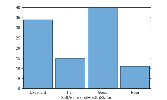
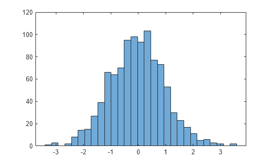
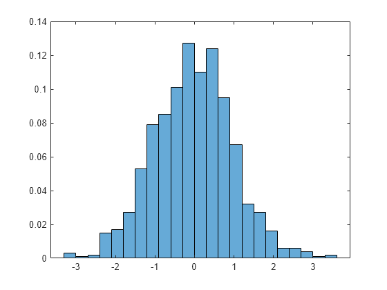
Generate 1,000 random numbers and create a histogram using the 'probability' normalization.
x = randn(1000,1);
h = histogram(x,'Normalization','probability')
h =
  Histogram with properties:

             Data: [1000×1 double]
           Values: [0.0030 1.0000e-03 0.0020 0.0150 0.0170 0.0270 0.0530 0.0790 0.0850 0.1010 0.1270 0.1100 0.1240 0.0950 0.0670 0.0320 0.0270 0.0160 0.0060 0.0060 0.0040 1.0000e-03 0.0020]
          NumBins: 23
         BinEdges: [-3.3000 -3.0000 -2.7000 -2.4000 -2.1000 -1.8000 -1.5000 -1.2000 -0.9000 -0.6000 -0.3000 0 0.3000 0.6000 0.9000 1.2000 1.5000 1.8000 2.1000 2.4000 2.7000 3 3.3000 3.6000]
         BinWidth: 0.3000
        BinLimits: [-3.3000 3.6000]
    Normalization: 'probability'
        FaceColor: 'auto'
        EdgeColor: [0.1294 0.1294 0.1294]

  Show all properties
Compute the sum of the bar heights. With this normalization, the height of each bar is equal to the probability of selecting an observation within that bin interval, and the height of all of the bars sums to 1.
S = sum(h.Values)
S =
1
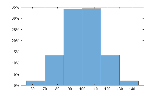
Generate 100,000 normally distributed random numbers. Use a standard deviation of 15 and a mean of 100.
x = 100 + 15*randn(1e5,1);
Plot a histogram of the random numbers. Scale and label the y-axis as percentages.
edges = 55:15:145;
histogram(x,edges,Normalization="percentage")
ytickformat("percentage")
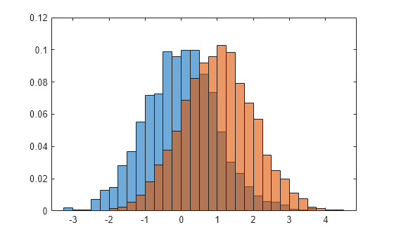
Generate two vectors of random numbers and plot a histogram for each vector in the same figure.
x = randn(2000,1);
y = 1 + randn(5000,1);
h1 = histogram(x);
hold on
h2 = histogram(y);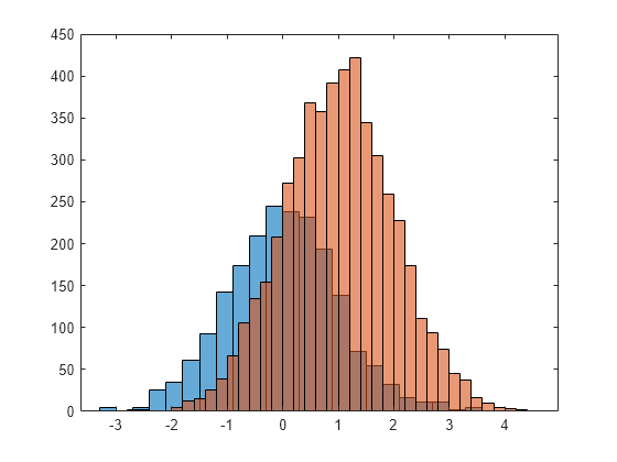
Since the sample size and bin width of the histograms are different, it is difficult to compare them. Normalize the histograms so that all of the bar heights add to 1, and use a uniform bin width.
h1.Normalization = 'probability';
h1.BinWidth = 0.25;
h2.Normalization = 'probability';
h2.BinWidth = 0.25;
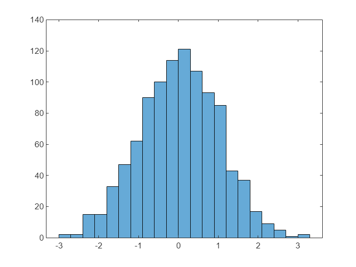
Create a histogram and return the Histogram object. Use the Histogram object to modify properties of the histogram after creating it.
x = randn(1000,1);
h = histogram(x)
h =
  Histogram with properties:

             Data: [1000×1 double]
           Values: [2 2 15 15 33 47 62 90 100 114 121 107 93 85 43 37 17 9 5 1 2]
          NumBins: 21
         BinEdges: [-3.0000 -2.7000 -2.4000 -2.1000 -1.8000 -1.5000 -1.2000 -0.9000 -0.6000 -0.3000 0 0.3000 0.6000 0.9000 1.2000 1.5000 1.8000 2.1000 2.4000 2.7000 3.0000 3.3000]
         BinWidth: 0.3000
        BinLimits: [-3.0000 3.3000]
    Normalization: 'count'
        FaceColor: 'auto'
        EdgeColor: [0 0 0]

  Show all properties
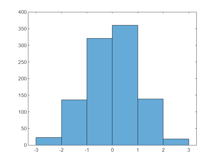
Specify the edges of the bins with a vector.
h.BinEdges = [-3:3];
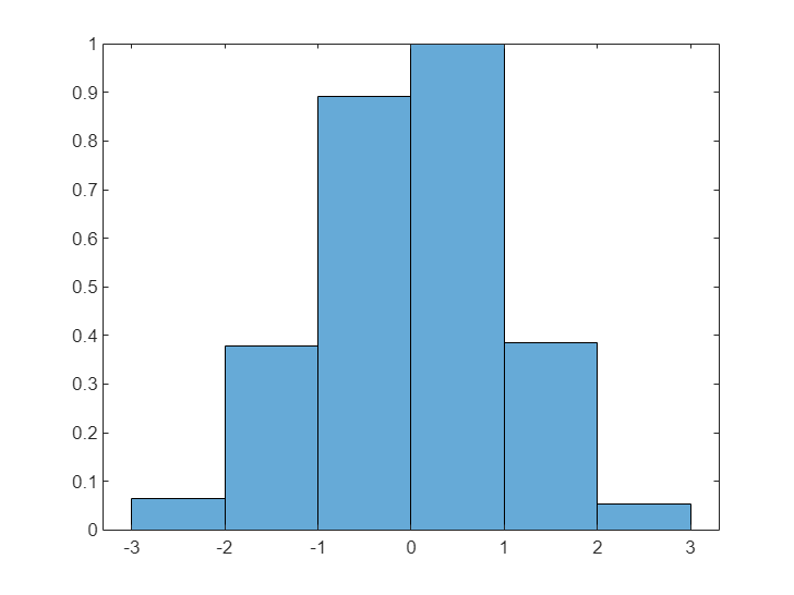
Normalize the bin counts so that the maximum bin count is 1.
h.BinCounts = h.BinCounts/max(h.BinCounts);
You can label each rectangular bar of a histogram with the number of elements it represents.
Create a histogram.
x = randn(1000,1);
h = histogram(x,5);
Return the bin counts and the x-axis position of each bin center.
counts = h.Values;
binEdges = h.BinEdges;
binCenters = binEdges(1:end-1) + diff(binEdges)/2;
Add a label to each bar that displays the number of elements it represents.
text(binCenters,counts,num2str(counts'),HorizontalAlignment="center",VerticalAlignment="bottom")

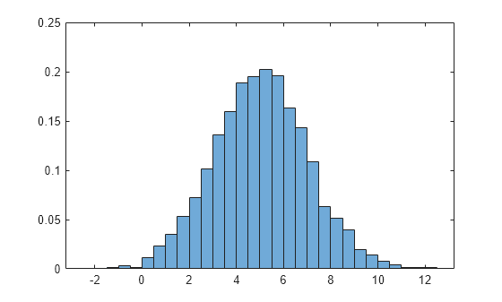
Generate 5,000 normally distributed random numbers with a mean of 5 and a standard deviation of 2. Plot a histogram with Normalization set to 'pdf' to produce an estimation of the probability density function.
x = 2*randn(5000,1) + 5;
histogram(x,'Normalization','pdf')
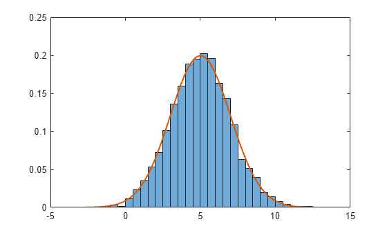
In this example, the underlying distribution for the normally distributed data is known. You can, however, use the 'pdf' histogram plot to determine the underlying probability distribution of the data by comparing it against a known probability density function.
The probability density function for a normal distribution with mean , standard deviation , and variance is
Overlay a plot of the probability density function for a normal distribution with a mean of 5 and a standard deviation of 2.
hold on
y = -5:0.1:15;
mu = 5;
sigma = 2;
f = exp(-(y-mu).^2./(2*sigma^2))./(sigma*sqrt(2*pi));
plot(y,f,'LineWidth',1.5)
Use the savefig function to save a histogram figure.
histogram(randn(10));
savefig('histogram.fig');
close gcf
Use openfig to load the histogram figure back into MATLAB®. openfig also returns a handle to the figure, h.
h = openfig('histogram.fig');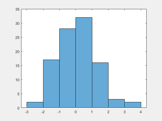
Use the findobj function to locate the correct object handle from the figure handle. This allows you to continue manipulating the original histogram object used to generate the figure.
y = findobj(h,'type','histogram')
y =
  Histogram with properties:

             Data: [10×10 double]
           Values: [2 17 28 32 16 3 2]
          NumBins: 7
         BinEdges: [-3 -2 -1 0 1 2 3 4]
         BinWidth: 1
        BinLimits: [-3 4]
    Normalization: 'count'
        FaceColor: 'auto'
        EdgeColor: [0.1294 0.1294 0.1294]

  Show all properties
Tips
Histogram plots created using
histogramhave a context menu in plot edit mode that enables interactive manipulations in the figure window. For example, you can use the context menu to interactively change the number of bins, align multiple histograms, or change the display order.When you add data tips to a histogram plot, they display the bin edges and bin count.