Main Content

DataDrivenMPC

Data-driven model predictive controller

Since R2026a

Description

A data-driven model predictive controller uses on a nonparametric model that relies on input/output time-domain data to directly (that is without explicit system identification) solve an MPC problem in real-time. To synthesize a data-driven MPC controller you use using data collected from an open loop experiment on the plant at a nominal operating point, using a persistently exciting input. All inputs are manipulated variables and all the outputs are measured.

Creation

Description

ddobj = DataDrivenMPC(dataU,dataY,Ts) creates a data-driven model predictive controller based on the input-output trajectory pair given by dataU and dataY, which are measured at the same time points with sample time of Ts.

example

Input Arguments

expand all

Plant input data from an open loop experiment, specified as a matrix with as many columns as the number of plant inputs, and as many rows as the number of samples. The data must be finite and uniformly sampled with the sample time Ts, given as a third argument.

Example: (0.5-rand(50,1))*2

Plant output data from an open loop experiment, specified as a matrix with as many columns as the number of plant outputs, and as many rows as the number of time steps. The data must be finite and uniformly sampled with the sample time Ts, given as a third argument.

Example: lsim(ss(-1,1,1,0),(0.5-rand(50,1))*2,0.1*(1:50)',0)

Sample time, specified as a positive finite scalar. This is the sample time used to collect dataU and dataY. This value is saved into the read-only Ts property of ddobj.

Example: 0.1

Properties

expand all

Sample time, specified as a positive finite scalar. This is the sample time used to collect dataU and dataY. This property is read-only and its value is set to the Ts input argument when ddobj is created.

Number of future steps used for prediction, specified as a positive integer. This is the horizon (from current time k to k+FutureSteps-1) over which the controller tries to minimize the cost and applies bounds on plant inputs and outputs. It should be long enough to capture the transient response and cover the significant dynamics of the system. A longer horizon requires the collection of more data points and increases both performance and computational requirements. A typical prediction horizon is 10 to 20 samples.

Note

The data-driven MPC FutureSteps property is similar to the classical MPC PredictionHorizon property. The main difference is that FutureSteps defines and interval that starts at the current time k while PredictionHorizon defines an interval that starts at time k+1.

After changing this property, check the values of the IsDataSufficient and IsPersistentlyExciting properties in the PersistentExcitation property of ddobj and make sure they remain true.

Example: ddobj.FutureSteps = 15

Number of past steps used for estimation, specified as a positive integer. This property indicates how many past samples must be used to sufficiently represent the current plant state. An accurate representation of the plant state is important for prediction, however, a large number of past steps requires the collection of more data points, increases computational requirements, and might lead to overfitting. A typical number of past steps is equal to or slightly greater than the value of PlantOrder.

After changing this property, check the values of the IsDataSufficient and IsPersistentlyExciting properties in the PersistentExcitation property of ddobj and make sure they remain true.

Example: ddobj.PastSteps = 4

Order of the plant model, specified as a positive integer. It is used by the software to check whether the input data is sufficiently long and persistently exciting. Set this value to the number of modes that, to your best knowledge, significantly contribute to the plant behavior.

After changing this property, check the values of the IsDataSufficient and IsPersistentlyExciting properties in the PersistentExcitation property of ddobj and make sure they remain true.

Example: ddobj.PlantOrder = 3

Dimensions of the plant model, returned as a read-only structure. This structure contains the following fields, which are used by the software to set up calculations and check whether the input data is sufficiently long and persistently exciting.

Number of plant inputs, returned as a positive integer. This field is read-only and its value is set to the number of columns of the dataU input argument when ddobj is created.

Number of plant outputs, returned as a positive integer. This field is read-only and its value is set to the number of columns of the dataY input argument when ddobj is created.

Depth of the Hankel matrix, returned as a positive integer. This field is read-only and its value is set to the sum of the FutureSteps and PastSteps properties when you change any of them. Multiplying HankelDepth by the sum of the number of inputs and outputs yields the number of rows of the stacked Hankel matrix, as defined in Data-Driven MPC Principles.

Number of columns of the Hankel matrix, returned as a positive integer. This field is read-only. When you change FutureSteps or PastSteps, the value of HankelWidth is set to the number of samples (see the PersistentExcitation.NumberOfSamples property), minus the value of the HankelDepth property, plus 1.

This property determines the length of the prediction vector, that is the number of Hankel variables, which are the most significant part of the decision variables of the resulting QP problem.

Number of slack variables on plant inputs, returned as a positive integer. This field is read-only and its value is set to the product between the NumberOfInputs and PastSteps properties when Weights.SlackPastU is finite. Slack variables can increase robustness to measurement noise and help avoiding infeasibility for problems with hard bounds.

Number of slack variables on plant inputs, returned as a positive integer. This field is read-only and its value is set to the product between the NumberOfOutputs and PastSteps properties when Weights.SlackPastY is finite. Slack variables can increase robustness to measurement noise and help avoiding infeasibility for problems with hard bounds.

Number of decision variables, returned as a positive integer. This field is read-only and its value is set to the sum of the HankelDepth, NumberOfSlackOnPastInputs, and NumberOfSlackOnPastOutputs properties when any of them changes.

Persistent excitation properties of the data used to create ddobj, returned as a read-only structure. This structure contains the following fields, which are used by the software to check whether the input data is sufficiently long and persistently exciting.

Number of samples, returned as a positive integer. This field is read-only and its value is set to the number of rows of the dataU and dataY input arguments when ddobj is created.

Minimum number of samples, returned as a positive integer. This field is read-only and its value is set to (Nu+1)(L+n)-1 whenever FutureSteps, PastSteps or PlantOrder changes. Here, Nu is the number of plant inputs, L is the value of the HankelDepth property, and n is the plant order.

If NumberOfSamples is less than MinimumNumberOfSamples, then the IsDataSufficient property is false.

Depth of the Hankel matrix, returned as a positive integer. This field is read-only and its value is set to the sum of the FutureSteps and PastSteps properties when you change any of them. Multiplying HankelDepth by the sum of the number of inputs and outputs yields the number of rows of the stacked Hankel matrix, as defined in Data-Driven MPC Principles.

Maximum number of rows for the Hankel matrix, returned as a positive integer. This field is read-only and its value is set to the floor of (L+1)/(Nu+1)-n whenever FutureSteps, PastSteps or PlantOrder changes. Here, Nu is the number of plant inputs, L is the value of the HankelDepth property, and n is the plant order.

If the value of the HankelDepth property exceeds the value of the MaximumHankelDepth property, then the value of the IsDataSufficient property is false.

Flag indicating whether the number of samples is sufficient for prediction, returned as either:

  • true — The number of samples is sufficient for prediction.

  • false — The number of samples is not sufficient for prediction. You can either use more samples in dataU and dataY or adjust FutureSteps, PastSteps and/or PlantOrder, depending on your design situation.

This property is true when the HankelDepth is not greater than MaximumHankelDepth, and NumberOfSamples is not smaller than MinimumNumberOfSamples.

Flag indicating whether the input is persistently exciting, returned as either:

  • true — The number of samples is persistently exciting.

  • false — The number of samples is not persistently exciting. Redesign your plant input signal so that it can sufficiently excite the relevant plant modes.

This property is true when the Hankel matrix has full row rank.

Condition number of the Hankel matrix, returned as a positive scalar. A large value is usually caused by insufficient input signal quality and might lead to poor prediction. For example, if the magnitude of the excitation of the plant modes is small compared to sensor noise, the resulting condition number of the Hankel matrix might be large. In this case, to improve the condition number, modify the excitation signal to increase the Signal to Noise Ratio (SNR).

Manipulated Variable (MV) bounds, specified as an ManipulatedVariables object with the Min, Max, RateMin and RateMax properties.

Note

Rates refer to the difference Δu(k)=u(k)-u(k-1). Constraints and weights based on derivatives du/dt of continuous-time input signals must be properly reformulated for the discrete-time difference Δu(k), using the approximation du/dt ≅ Δu(k)/Ts.

Each property is a matrix with Dimensions.NumberOfInputs columns and up to FutureSteps rows.

Lower bounds for the manipulated variables, specified as matrix in which each column vector corresponds to a manipulated variable.

To use the same bound across the prediction horizon, specify a row vector containing a scalar bound for each manipulated variable. By default, Min is a row vector in which each element is -Inf.

To vary the bound over the prediction horizon from the current time k to time k+FutureSteps-1, specify a column vector of up to FutureSteps values for each manipulated variable. If you specify fewer than FutureSteps values, the final bound is used for the remaining steps of the prediction horizon.

Example: ddobj.ManipulatedVariables.Min = [-1 -1 -1];

Upper bounds for the manipulated variables, specified as matrix in which each column vector corresponds to a manipulated variable.

To use the same bound across the prediction horizon, specify a row vector containing a scalar bound for each manipulated variable. By default, Max is a row vector in which each element is Inf.

To vary the bound over the prediction horizon from the current time k to time k+FutureSteps-1, specify a column vector of up to FutureSteps values for each manipulated variable. If you specify fewer than FutureSteps values, the final bound is used for the remaining steps of the prediction horizon.

Example: ddobj.ManipulatedVariables.Max = [1 1 1];

Lower bounds for the rate of change of the manipulated variables, specified as matrix in which each column vector corresponds to a manipulated variable.

To use the same bound across the prediction horizon, specify a row vector containing a scalar bound for each manipulated variable. By default, RateMin is a row vector in which each element is -Inf.

To vary the bound over the prediction horizon from the current time k to time k+FutureSteps-1, specify a column vector of up to FutureSteps values for each manipulated variable. If you specify fewer than FutureSteps values, the final bound is used for the remaining steps of the prediction horizon.

Example: ddobj.ManipulatedVariables.RateMin = [-10 -10 -10];

Upper bounds for the rate of change of the manipulated variables, specified as matrix in which each column vector corresponds to a manipulated variable.

To use the same bound across the prediction horizon, specify a row vector containing a scalar bound for each manipulated variable. By default, RateMax is a row vector in which each element is Inf.

To vary the bound over the prediction horizon from the current time k to time k+FutureSteps-1, specify a column vector of up to FutureSteps values for each manipulated variable. If you specify fewer than FutureSteps values, the final bound is used for the remaining steps of the prediction horizon.

Example: ddobj.ManipulatedVariables.RateMax = [10 10 10];

Output Variable (OV) bounds, specified as an OutputVariables object with the Min and Max properties.

Each property is a matrix with Dimensions.NumberOfOutputs columns and up to FutureSteps rows.

Lower bounds for the output variables, specified as matrix in which each column vector corresponds to an output variable.

To use the same bound across the prediction horizon, specify a row vector containing a scalar bound for each manipulated variable. By default, Min is a row vector in which each element is -Inf.

To vary the bound over the prediction horizon from the current time k to time k+FutureSteps-1, specify a column vector of up to FutureSteps values for each manipulated variable. If you specify fewer than FutureSteps values, the final bound is used for the remaining steps of the prediction horizon.

Example: ddobj.OutputVariables.Min = [-2 -2];

Lower bounds for the output variables, specified as matrix in which each column vector corresponds to an output variable.

To use the same bound across the prediction horizon, specify a row vector containing a scalar bound for each manipulated variable. By default, Min is a row vector in which each element is Inf.

To vary the bound over the prediction horizon from the current time k to time k+FutureSteps-1, specify a column vector of up to FutureSteps values for each manipulated variable. If you specify fewer than FutureSteps values, the final bound is used for the remaining steps of the prediction horizon.

Example: ddobj.OutputVariables.Max = [2 2];

Standard cost function tuning weights, specified as a Weights object with the following properties.

Weights for the manipulated variables, which penalize large values of the control action, specified as matrix in which each column vector corresponds to a manipulated variable.

To use the same weight across the prediction horizon, specify a row vector containing a weight for each manipulated variable. By default, ManipulatedVariables is a row vector in which each element is 0.

To vary the weight over the prediction horizon from the current time k to time k+FutureSteps-1, specify a column vector of up to FutureSteps values for each manipulated variable. If you specify fewer than FutureSteps values, the final weight is used for the remaining steps of the prediction horizon.

Example: ddobj.Weights.ManipulatedVariables = [0.1 0.2]

Weights for the manipulated variable rates, which penalize large changes in control moves, specified as matrix in which each column vector corresponds to a manipulated variable.

To use the same weight across the prediction horizon, specify a row vector containing a weight for each manipulated variable. By default, ManipulatedVariablesRate is a row vector in which each element is 0.1.

To vary the weight over the prediction horizon from the current time k to time k+FutureSteps-1, specify a column vector of up to FutureSteps values for each manipulated variable. If you specify fewer than FutureSteps values, the final weight is used for the remaining steps of the prediction horizon.

Manipulated variable rate tuning weights, , specified as a row vector or array of nonnegative values. The default weight for all manipulated variable rates is 0.1.

Note

It is best practice to use nonzero manipulated variable rate weights. If all manipulated variable rate weights are strictly positive, the resulting QP problem is strictly convex. If some weights are zero, the QP Hessian could be positive semidefinite. To keep the QP problem strictly convex, when the condition number of the Hessian matrix KΔU is larger than 1012, the quantity 10*sqrt(eps) is added to each diagonal term. See Cost Function.

Example: ddobj.Weights.ManipulatedVariablesRate = [0.1 0.1]

Weights for the output variables, which penalize large values of the plant outputs, specified as matrix in which each column vector corresponds to an output variable.

To use the same weight across the prediction horizon, specify a row vector containing a weight for each output variable. By default, OutputVariables is a row vector in which each element is 1.

To vary the weight over the prediction horizon from the current time k to time k+FutureSteps-1, specify a column vector of up to FutureSteps values for each manipulated variable. If you specify fewer than FutureSteps values, the final weight is used for the remaining steps of the prediction horizon.

Example: ddobj.Weights.OutputVariables = [1 1]

Weight for the predictor vector (that is the vector of the Hankel decision variables), specified as a positive scalar. This weight penalizes larges values of the Hankel matrix elements, and is indicated by σα in Data-Driven MPC Formulation. Setting this property to 0 effectively removes regularization and allows vary high values of α, which typically leads to numerical issue in the optimization algorithm. Conversely, higher values of this property can distort the overall cost function of your controller.

Example: mpcobj.Weights.HankelVariables = 1e-3

Weight for the slack variables applied to the past outputs, specified as a positive scalar. This weight softens the equality constraints applied to the past output trajectory, and is indicated by σy in Data-Driven MPC Formulation. Lower values can increase robustness to sensor noise and small nonlinearities. Setting this property to inf removes the corresponding slack variables.

Example: mpcobj.Weights.SlackPastY = 1e6

Weight for slack variables applied to past inputs, specified as a positive scalar. This weight softens the equality constraints applied to the past input trajectory, and is indicated by σu in Data-Driven MPC Formulation. Lower values can increase robustness to sensor noise and small nonlinearities. Setting this property to inf removes the corresponding slack variables.

Example: mpcobj.Weights.SlackPastU = 1e6

Optimization information for the solver, specified as a structure with the following field.

For more information on QP solvers, see QP Solvers for Linear MPC.

Solver algorithm, specified as 'active-set'. This algorithm solves the QP problem using the KWIK active-set algorithm.

Example: ddobj.Optimizer.Solver = 'active-set'

Solver options, specified as an ActiveSet options object. For more information, see the Solver property and QP Solvers for Linear MPC.

Object Functions

mpcmoveCompute optimal control action and update controller states
simSimulate an MPC controller in closed loop with a linear plant

Examples

collapse all

In this example you create a DataDrivenMPC object, validate its internal model, and then simulate the controller in closed loop.

Create a plant model and collect input and output data

To collect input and output data, first define random, strictly causal, continuous-time plant with two outputs, three inputs, and four states. For more information on creating random systems, see rss.

nx = 4; ny = 2; nu = 3;
sys = rss(nx,ny,nu); sys.D = 0;

Note that for data-driven MPC design, all inputs must be manipulated variables.

Define an initial state.

x0 = zeros(4,1);

Define a sampling time of 0.1 seconds and define a column time vector of 100 samples starting from t = 1 second.

Ts = 0.1;
N = 100;
t = (1:N)'*Ts;

Create a random input signal. Inputs with a random component are typically persistently exciting.

dataU = (0.5-rand(length(t),nu))*2;

To collect output data, simulate the plant model using the lsim function. Supply as argument the plant model, the input data, the time vector, and the initial state created in the previous steps.

dataY = lsim(sys,dataU,t,x0);

If you have already have plant input and output data collected from experiments, then this step not necessary, as you can directly use your existing data to design your data-driven MPC controller.

Create a data-driven MPC controller

Create a DataDrivenMPC object using the input and output data as well as the sample time.

ddobj = DataDrivenMPC(dataU,dataY,Ts)
ddobj = 
  DataDrivenMPC with properties:

                      Ts: 0.1000
             FutureSteps: 1
               PastSteps: 1
              PlantOrder: 1
              Dimensions: [1×1 struct]
    PersistentExcitation: [1×1 struct]
    ManipulatedVariables: [1×1 mpc.internal.ddmpc.ManipulatedVariables]
         OutputVariables: [1×1 mpc.internal.ddmpc.OutputVariables]
                 Weights: [1×1 mpc.internal.ddmpc.Weights]
            Optimization: [1×1 mpc.internal.ddmpc.Optimization]

Set the number of steps used for prediction, FutureSteps, the number of steps used for estimation, PastSteps, and the plant order. The software uses the plant order to check whether the input data is sufficiently long and persistently exciting.

ddobj.FutureSteps = 21; 
ddobj.PastSteps = 4;
ddobj.PlantOrder = nx;

Check the PersistentExcitation property to make sure the last two properties are true. If not, you might need to provide more data (assuming the number of prediction and estimation steps does not change) or redesign the excitation signal.

ddobj.PersistentExcitation
ans = struct with fields:
           NumberOfSamples: 100
    MinimumNumberOfSamples: 115
               HankelDepth: 25
        MaximumHankelDepth: 21
          IsDataSufficient: 0
    IsPersistentlyExciting: 0
     HankelConditionNumber: 12.5931

Define bounds for the manipulated variables and their rate.

ddobj.ManipulatedVariables.Min = -5*ones(1,nu);
ddobj.ManipulatedVariables.Max = 5*ones(1,nu);
ddobj.ManipulatedVariables.RateMin = -0.5*ones(1,nu);
ddobj.ManipulatedVariables.RateMax = 0.5*ones(1,nu);

Validate prediction model

Create a time vector for validation.

L = ddobj.PastSteps + ddobj.FutureSteps;
t_val = (1:L)'*Ts;

Create a random input signal for validation.

dataU_val = (0.5-rand(L,nu))*2;

To collect output data for validation, simulate the plant model you created in the first step, using the validation input data, time vector and initial state as additional input arguments.

dataY_val = lsim(sys,dataU_val,t_val,x0);

Use the checkPrediction function to check whether the internal model in ddobj can predict the validation output data.

checkPrediction(ddobj,dataU_val,dataY_val);

Figure contains 2 axes objects. Axes object 1 with title Prediction Validation, xlabel time, ylabel y(1) contains 2 objects of type line. One or more of the lines displays its values using only markers These objects represent measured output, predicted output. Axes object 2 with xlabel time, ylabel y(2) contains 2 objects of type line. One or more of the lines displays its values using only markers These objects represent measured output, predicted output.

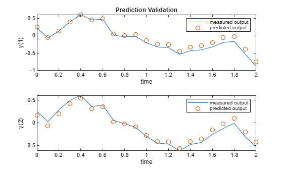
The predicted output acceptably matches the validation output (dataY_val).

Simulate the controller in closed loop

Use a step as a reference signal for all outputs.

ref = ones(1,ny);

Perform a closed loop simulation using the internal prediction model. For more information, see sim.

sim(ddobj,N/2,ref);

Figure contains 3 axes objects. Axes object 1 with title Data-Driven MPC: Plant Inputs contains an object of type stair. Axes object 2 contains an object of type stair. Axes object 3 contains an object of type stair.

Figure contains 2 axes objects. Axes object 1 with title Data-Driven MPC: Plant Outputs contains an object of type stair. Axes object 2 contains an object of type stair.

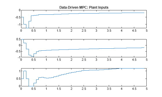
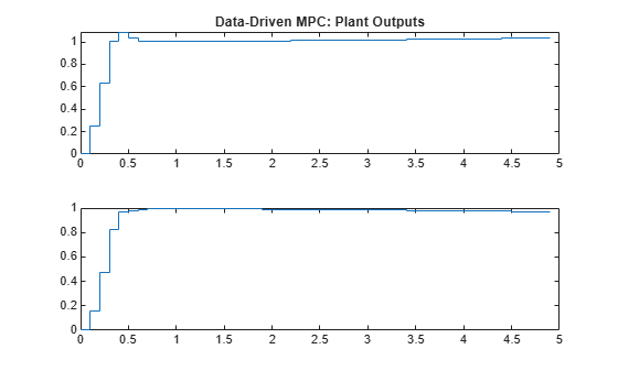
The controller is able to track the reference.

Calculate optimal input move

Create a step reference signal for all outputs over ddobj.FutureSteps steps.

yref = repmat(ref,ddobj.FutureSteps,1);

Create a state object.

stateobj = DataDrivenMPCState(ddobj);

To calculate the optimal input move use mpcmove. Supply as input arguments the DataDrivenMPC object, the state object, the measured plant inputs and outputs at the previous control interval and the reference signal.

 mv = mpcmove(ddobj,stateobj,zeros(nu,1),zeros(ny,1),yref)
mv = 3×1

   -0.5000
    0.5000
    0.5000

You can simulate the controller in closed loop against a linear or nonlinear plant using mpcmove in a for loop.

Version History

Introduced in R2026a