FrequencyStructuralResults
Frequency response structural solution and derived quantities
Description
A FrequencyStructuralResults object contains the
displacement, velocity, and acceleration in a form convenient for plotting and
postprocessing.
Displacement, velocity, and acceleration are reported for the nodes of the triangular or
tetrahedral mesh generated by generateMesh. The displacement, velocity, and
acceleration values at the nodes appear as FEStruct objects in the
Displacement, Velocity, and
Acceleration properties. The properties of these objects contain the
components of the displacement, velocity, and acceleration at the nodal locations.
To evaluate the stress, strain, von Mises stress, principal stress, and principal strain
at the nodal locations, use evaluateStress,
evaluateStrain,
evaluateVonMisesStress, evaluatePrincipalStress, and evaluatePrincipalStrain, respectively.
To evaluate the reaction forces on a specified boundary, use evaluateReaction.
To interpolate the displacement, velocity, acceleration, stress, strain, and von Mises
stress to a custom grid, such as the one specified by meshgrid, use interpolateDisplacement, interpolateVelocity,
interpolateAcceleration, interpolateStress,
interpolateStrain,
and interpolateVonMisesStress, respectively.
For a frequency response model with damping, the results are complex. Use functions such
as abs and angle to obtain real-valued results, such as
the magnitude and phase. See Solve Frequency Response Structural Problem with Damping.
Creation
Solve a frequency response problem by using the solve function. This function returns a frequency response structural solution
as a FrequencyStructuralResults object.
Properties
Object Functions
evaluateStress | Evaluate stress for dynamic structural analysis problem |
evaluateStrain | Evaluate strain for dynamic structural analysis problem |
evaluateVonMisesStress | Evaluate von Mises stress for dynamic structural analysis problem |
evaluateReaction | Evaluate reaction forces on boundary |
evaluatePrincipalStress | Evaluate principal stress at nodal locations |
evaluatePrincipalStrain | Evaluate principal strain at nodal locations |
interpolateDisplacement | Interpolate displacement at arbitrary spatial locations |
interpolateVelocity | Interpolate velocity at arbitrary spatial locations for all time or frequency steps for dynamic structural problem |
interpolateAcceleration | Interpolate acceleration at arbitrary spatial locations for all time or frequency steps for dynamic structural problem |
interpolateStress | Interpolate stress at arbitrary spatial locations |
interpolateStrain | Interpolate strain at arbitrary spatial locations |
interpolateVonMisesStress | Interpolate von Mises stress at arbitrary spatial locations |
Examples
Solve a frequency response problem with damping. The resulting displacement values are complex. To obtain the magnitude and phase of displacement, use the abs and angle functions, respectively. To speed up computations, solve the model using the results of modal analysis.
Modal Analysis
Create a geometry representing a thin plate.
gm = multicuboid(10,10,0.025);
Create an femodel object for modal analysis and include the geometry in the model.
model = femodel(AnalysisType="structuralModal", ...
                Geometry=gm);
Generate a mesh.
model = generateMesh(model);
Specify Young's modulus, Poisson's ratio, and the mass density of the material.
model.MaterialProperties = ...
    materialProperties(YoungsModulus=2E11, ...
                       PoissonsRatio=0.3, ...
                       MassDensity=8000);
Identify faces for applying boundary constraints and loads by plotting the geometry with the face and edge labels.
pdegplot(model.Geometry,FaceLabels="on",FaceAlpha=0.5)
figure
pdegplot(model.Geometry,EdgeLabels="on",FaceAlpha=0.5)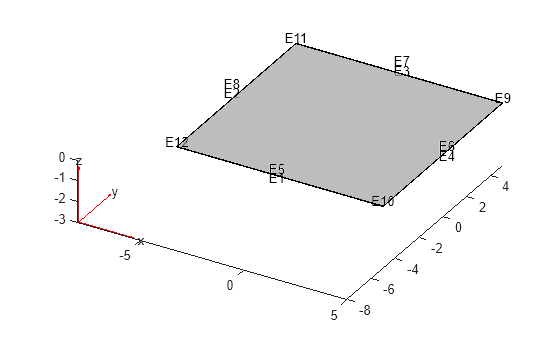
Specify constraints on the sides of the plate (faces 3, 4, 5, and 6) to prevent rigid body motions.
model.FaceBC([3,4,5,6]) = faceBC(Constraint="fixed");Solve the problem for the frequency range from -Inf to 12*pi.
Rm = solve(model,FrequencyRange=[-Inf,12*pi]);
Frequency Response Analysis
Switch the analysis type of the model to frequency response.
model.AnalysisType = "structuralFrequency";Specify the pressure loading on top of the plate (face 2) to model an ideal impulse excitation. In the frequency domain, this pressure pulse is uniformly distributed across all frequencies.
model.FaceLoad(2) = faceLoad(Pressure=1E2);
First, solve the problem without damping.
flist = [0,1,1.5,linspace(2,3,100),3.5,4,5,6]*2*pi;
RfrModalU = solve(model,flist,ModalResults=Rm);
Now, solve the problem with damping equal to 2% of critical damping for all modes.
RfrModalAll = solve(model,flist, ...
                    ModalResults=Rm, ...
                    DampingZeta=0.02);
Solve the same problem with frequency-dependent damping. In this example, use the solution frequencies from flist and damping values between 1% and 10% of critical damping.
omega = flist;
zeta = linspace(0.01,0.1,length(omega));
zetaW = @(omegaMode) interp1(omega,zeta,omegaMode);

RfrModalFD = solve(model,flist, ...
                   ModalResults=Rm, ...
                   DampingZeta=zetaW);
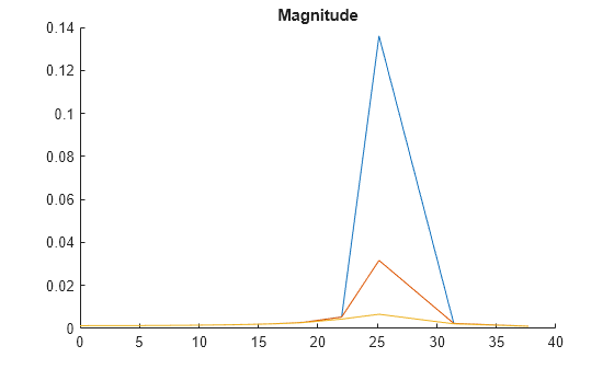
Interpolate the displacement at the center of the top surface of the plate for all three cases.
iDispU = interpolateDisplacement(RfrModalU,[0;0;0.025]);
iDispAll = interpolateDisplacement(RfrModalAll,[0;0;0.025]);
iDispFD = interpolateDisplacement(RfrModalFD,[0;0;0.025]);
Plot the magnitude of the displacement.
figure
hold on
plot(RfrModalU.SolutionFrequencies,abs(iDispU.Magnitude));
plot(RfrModalAll.SolutionFrequencies,abs(iDispAll.Magnitude));
plot(RfrModalFD.SolutionFrequencies,abs(iDispFD.Magnitude));
title("Magnitude")
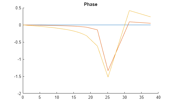
Plot the phase of the displacement.
figure
hold on
plot(RfrModalU.SolutionFrequencies,angle(iDispU.Magnitude));
plot(RfrModalAll.SolutionFrequencies,angle(iDispAll.Magnitude));
plot(RfrModalFD.SolutionFrequencies,angle(iDispFD.Magnitude));
title("Phase")
Version History
Introduced in R2019b
See Also
Functions
solve|evaluateStress|evaluateStrain|evaluateVonMisesStress|evaluateReaction|evaluatePrincipalStress|evaluatePrincipalStrain|interpolateDisplacement|interpolateVelocity|interpolateAcceleration|interpolateStress|interpolateStrain|interpolateVonMisesStress