interpolateMagneticFlux
Interpolate magnetic flux density in magnetostatic result at arbitrary spatial locations
Since R2021a
Syntax
Description
Bintrp = interpolateMagneticFlux(magnetostaticresults,xq,yq)xq and yq.
Bintrp = interpolateMagneticFlux(magnetostaticresults,xq,yq,zq)xq, yq, and
zq.
Bintrp = interpolateMagneticFlux(magnetostaticresults,querypoints)querypoints.
Examples
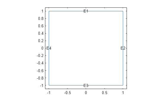
Create a square geometry and plot it with the edge labels.
R1 = [3,4,-1,1,1,-1,1,1,-1,-1]';
g = decsg(R1,'R1',('R1')');
pdegplot(g,EdgeLabels="on")
xlim([-1.1 1.1])
ylim([-1.1 1.1])
Create an femodel object for magnetostatic analysis and include the geometry into the model.
model = femodel(AnalysisType="magnetostatic", ...
                Geometry=g);
Specify the vacuum permeability in the SI system of units.
model.VacuumPermeability = 1.2566370614E-6;
Specify the relative permeability of the material.
model.MaterialProperties = ...
    materialProperties(RelativePermeability=5000);
Apply the magnetic potential boundary conditions on the boundaries of the square.
model.EdgeBC([1 3]) = edgeBC(MagneticPotential=0);
model.EdgeBC([2 4]) = edgeBC(MagneticPotential=0.01);
Specify the current density for the entire geometry.
model.FaceLoad = faceLoad(CurrentDensity=0.5);
Generate the mesh.
model = generateMesh(model);
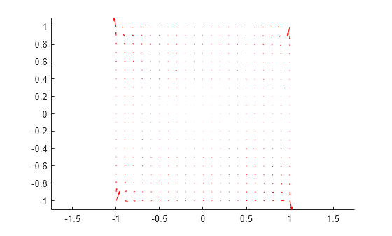
Solve the problem and plot the magnetic flux density.
R = solve(model);
pdeplot(R.Mesh,FlowData=[R.MagneticFluxDensity.Bx ...
                         R.MagneticFluxDensity.By])
axis equal
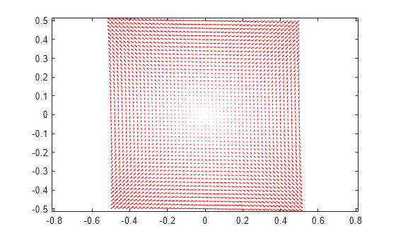
Interpolate the resulting electric flux density to a grid covering the central portion of the geometry, for x and y from -0.5 to 0.5.
v = linspace(-0.5,0.5,51);
[X,Y] = meshgrid(v);
Bintrp = interpolateMagneticFlux(R,X,Y)
Bintrp =
  FEStruct with properties:

    Bx: [2601×1 double]
    By: [2601×1 double]
Reshape Bintrp.Bx and Bintrp.By and plot the resulting magnetic flux density.
BintrpX = reshape(Bintrp.Bx,size(X));
BintrpY = reshape(Bintrp.By,size(Y));
figure
quiver(X,Y,BintrpX,BintrpY,Color="red")
axis equal
Alternatively, you can specify the grid by using a matrix of query points.
querypoints = [X(:),Y(:)]';
Bintrp = interpolateMagneticFlux(R,querypoints);
Create an femodel object for magnetostatic analysis and include a geometry of a plate with a hole into the model.
model = femodel(AnalysisType="magnetostatic", ...
                Geometry="PlateHoleSolid.stl");
Plot the geometry.
pdegplot(model.Geometry,FaceLabels="on",FaceAlpha=0.3)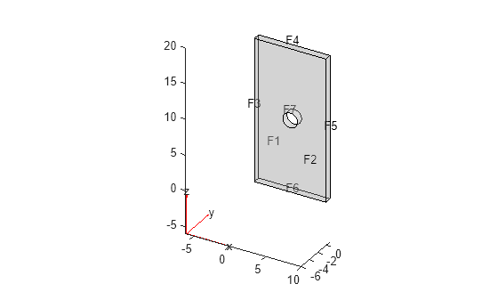
Specify the vacuum permeability value in the SI system of units.
model.VacuumPermeability = 1.2566370614E-6;
Specify the relative permeability of the material.
model.MaterialProperties = ...
    materialProperties(RelativePermeability=5000);
Specify the current density for the entire geometry.
model.CellLoad = cellLoad(CurrentDensity=[0;0;0.5]);
Apply the magnetic potential boundary conditions on the side faces and the face bordering the hole.
model.FaceBC(3:6) = faceBC(MagneticPotential=[0;0;0]);
model.FaceBC(7) = faceBC(MagneticPotential=[0;0;0.01]);
Generate a mesh.
model = generateMesh(model);
Solve the problem.
R = solve(model)
R =
  MagnetostaticResults with properties:

      MagneticPotential: [1×1 FEStruct]
          MagneticField: [1×1 FEStruct]
    MagneticFluxDensity: [1×1 FEStruct]
                   Mesh: [1×1 FEMesh]
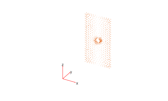
Plot the magnetic flux density.
pdeplot3D(R.Mesh,FlowData=[R.MagneticFluxDensity.Bx ...
                           R.MagneticFluxDensity.By ...
                           R.MagneticFluxDensity.Bz])
Interpolate the resulting magnetic flux density to a grid covering the central portion of the geometry, for x, y, and z.
x = linspace(3,7,5);
y = linspace(0,1,5);
z = linspace(8,12,5);
[X,Y,Z] = meshgrid(x,y,z);
Bintrp = interpolateMagneticFlux(R,X,Y,Z)
Bintrp =
  FEStruct with properties:

    Bx: [125×1 double]
    By: [125×1 double]
    Bz: [125×1 double]
Reshape Bintrp.Bx, Bintrp.By, and Bintrp.Bz.
BintrpX = reshape(Bintrp.Bx,size(X));
BintrpY = reshape(Bintrp.By,size(Y));
BintrpZ = reshape(Bintrp.Bz,size(Z));
Plot the resulting magnetic flux density.
figure
quiver3(X,Y,Z,BintrpX,BintrpY,BintrpZ,Color="red")
view([30 10])
view([10 15])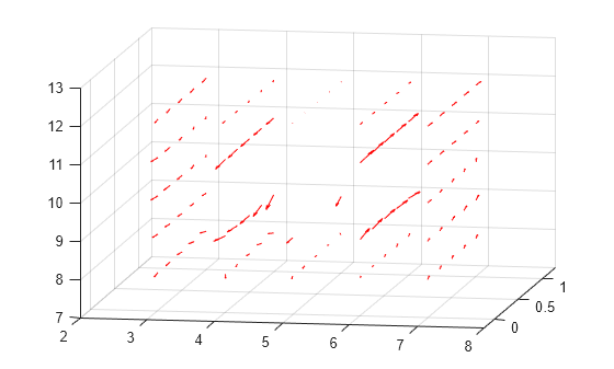
Input Arguments
Solution of a magnetostatic problem, specified as a MagnetostaticResults object. Create magnetostaticresults
using the solve function.
x-coordinate query points, specified as a real array.
interpolateMagneticFlux evaluates the magnetic flux density at the
2-D coordinate points [xq(i) yq(i)] or at the 3-D coordinate points
[xq(i) yq(i) zq(i)] for every i. Because of
this, xq, yq, and (if present)
zq must have the same number of entries.
interpolateMagneticFlux converts the query points to column
vectors xq(:) and yq(:). It returns magnetic flux
density as a column vector of the same size. To ensure that the dimensions of the
returned solution are consistent with the dimensions of the original query points, use
reshape. For example, use BintrpX =
reshape(Bintrp.Bx,size(xq)).
Example: xq = [0.5 0.5 0.75 0.75]
Data Types: double
y-coordinate query points, specified as a real array.
interpolateMagneticFlux evaluates the magnetic flux density at the
2-D coordinate points [xq(i) yq(i)] or at the 3-D coordinate points
[xq(i) yq(i) zq(i)] for every i. Because of
this, xq, yq, and (if present)
zq must have the same number of entries.
interpolateMagneticFlux converts the query points to column
vectors xq(:), yq(:), and (if present)
zq(:). It returns magnetic flux density as a column vector of the
same size. To ensure that the dimensions of the returned solution are consistent with
the dimensions of the original query points, use reshape. For
example, use BintrpY = reshape(Bintrp.By,size(yq)).
Example: yq = [1 2 0 0.5]
Data Types: double
z-coordinate query points, specified as a real array.
interpolateMagneticFlux evaluates the magnetic flux density at the
3-D coordinate points [xq(i) yq(i) zq(i)]. Therefore,
xq, yq, and zq must have
the same number of entries.
interpolateMagneticFlux converts the query points to column
vectors xq(:), yq(:), and
zq(:). It returns magnetic flux density values as a column vector of
the same size. To ensure that the dimensions of the returned solution are consistent
with the dimensions of the original query points, use reshape. For
example, use BintrpZ = reshape(Bintrp.Bz,size(zq)).
Example: zq = [1 1 0 1.5]
Data Types: double
Query points, specified as a real matrix with two rows for 2-D geometry or three
rows for 3-D geometry. interpolateMagneticFlux evaluates the magnetic
flux density at the coordinate points querypoints(:,i) for every
i, so each column of querypoints contains
exactly one 2-D or 3-D query point.
Example: For a 2-D geometry, querypoints = [0.5 0.5 0.75 0.75; 1 2 0
0.5]
Data Types: double
Output Arguments
Magnetic flux density at query points, returned as an FEStruct
object with the properties representing the spatial components of the magnetic flux
density at the query points. For query points that are outside the geometry,
Bintrp.Bx(i), Bintrp.By(i), and
Bintrp.Bz(i) are NaN. Properties of an
FEStruct object are read-only.
Version History
Introduced in R2021a
See Also
Objects
Functions
MATLAB Command
You clicked a link that corresponds to this MATLAB command:
Run the command by entering it in the MATLAB Command Window. Web browsers do not support MATLAB commands.
Select a Web Site
Choose a web site to get translated content where available and see local events and offers. Based on your location, we recommend that you select: .
You can also select a web site from the following list
How to Get Best Site Performance
Select the China site (in Chinese or English) for best site performance. Other MathWorks country sites are not optimized for visits from your location.
Americas
- América Latina (Español)
- Canada (English)
- United States (English)
Europe
- Belgium (English)
- Denmark (English)
- Deutschland (Deutsch)
- España (Español)
- Finland (English)
- France (Français)
- Ireland (English)
- Italia (Italiano)
- Luxembourg (English)
- Netherlands (English)
- Norway (English)
- Österreich (Deutsch)
- Portugal (English)
- Sweden (English)
- Switzerland
- United Kingdom (English)