phased.BackscatterSonarTarget

Sonar target backscatter

Description

The phased.BackscatterSonarTarget System object™ models the backscattering of a signal from an underwater or surface target. Backscattering is a special case of sonar target scattering when the incident and reflected angles are the same. This type of scattering applies to monostatic sonar configurations. The sonar target strength (TS) determines the backscattering response of a target to an incoming signal. This object lets you specify an angle-dependent sonar target strength model that covers a range of incident angles.

The object lets you specify the target strength as an array of values at discrete azimuth and elevation points. The object interpolates values for incident angles between array points.

You can employ one of four Swerling models to generate random fluctuations in the target strength. Choose the fluctuation model using the Model property. Then, use the SeedSource and Seed properties to control the fluctuations.

To model a backscattered reflected sonar signal:

1. Create the phased.BackscatterSonarTarget object and set its properties.

2. Call the object with arguments, as if it were a function.

To learn more about how System objects work, see What Are System Objects?

Creation

Syntax

target = phased.BackscatterSonarTarget

target = phased.BackscatterSonarTarget(Name=Value)

Description

target = phased.BackscatterSonarTarget creates a backscatter sonar target System object, target.

target = phased.BackscatterSonarTarget(Name=Value) creates a backscatter sonar target System object, target, with each specified property Name set to the specified Value. You can specify additional name and value arguments in any order as (Name1=Value1,...,NameN=ValueN).

Properties

Unless otherwise indicated, properties are nontunable, which means you cannot change their values after calling the object. Objects lock when you call them, and the release function unlocks them.

If a property is tunable, you can change its value at any time.

For more information on changing property values, see System Design in MATLAB Using System Objects.

target — Backscatter sonar target

phased.BackscatterSonarTarget System object

Backscatter sonar target, specified as a phased.BackscatterSonarTarget System object.

AzimuthAngles — Target strength azimuth angles

[-180:180] (default) | real-valued 1-by-P row vector | real-valued P-by-1 column vector

Target strength azimuth angles, specified as a real-valued 1-by-P row vector or P-by-1 column vector. These angles define the azimuth coordinates of each column of the matrix specified by the TSPattern property. P must be greater than two. Angle units are in degrees.

Example: [-45:0.1:45]

Data Types: double

ElevationAngles — Elevation angles

[-90:90] (default) | real-valued 1-by-Q row vector | real-valued Q-by-1 column vector

Target strength elevation angles, specified as a real-valued 1-by-Q row vector or Q-by-1 column vector. These angles define the elevation coordinates of each row of the matrix specified by the TSPattern property. Q must be greater than two. Angle units are in degrees.

Example: [-30:0.1:30]

Data Types: double

TSPattern — Sonar target strength pattern

zeros(181,361) (default) | Q-by-P real-valued matrix | Q-by-P-by-M real-valued array | 1-by-P real-valued vector | M-by-P real-valued matrix

Sonar target strength (TS) pattern, specified as a real-valued Q-by-P matrix or Q-by-P-by-M array. Q is the length of the vector in the ElevationAngles property. P is the length of the vector in the AzimuthAngles property. M is the number of target patterns. The number of patterns corresponds to the number of signals passed into the step method. You can, however, use a single pattern to model multiple signals reflecting from a single target. Pattern units are dB.

You can also specify the pattern as a function only of azimuth for a single elevation. In this case, specify the pattern as either a 1-by-P vector or an M-by-P matrix. Each row is a separate pattern.

Example: [1,2;3,4]

Data Types: double

Model — Target fluctuation model

"Nonfluctuating" (default) | "Swerling1" | "Swerling2" | "Swerling3" | "Swerling4"

Target fluctuation model, specified as "Nonfluctuating", "Swerling1", "Swerling2", "Swerling3", or "Swerling4". If you set this property to a value other than "Nonfluctuating", use the update input argument when calling the step method.

Example: "Swerling3"

Data Types: char

SeedSource — Seed source of random number generator for TS fluctuation model

"Auto" (default) | "Property"

Seed source of random number generator for TS fluctuation model, specified as "Auto" or "Property". When you set this property to "Auto", the System object generates random numbers using the default MATLAB^® random number generator. When you set this property to "Property", you specify the random number generator seed using the Seed property. This property applies when you set the Model property to"Swerling1", "Swerling2", "Swerling3", or "Swerling4". When you use this object with Parallel Computing Toolbox™ software, you set this property to "Auto".

Example: "Property"

Data Types: char

Seed — Random number generator seed

0 (default) | nonnegative integer less than 2³²

Random number generator seed, specified as a nonnegative integer less than 2³².

Example: 32301

Dependencies

To enable this property, set the SeedSource property to "Property".

Data Types: double

Usage

Syntax

refl_sig = target(sig,ang)

refl_sig = target(sig,ang,update)

Description

refl_sig = target(sig,ang) returns the reflected signal, refl_sig, of an incident sonar signal, sig, arriving at the target from the angle, ang.

refl_sig = target(sig,ang,update) uses update to control whether to update the target strength (TS) values. This syntax applies when you set the Model property to one of the fluctuating TS models: "Swerling1", "Swerling2", "Swerling3", or "Swerling4". If update is true, a new TS value is generated. If update is false, the previous TS value is used.

Note

The object performs an initialization the first time the object is executed. This initialization locks nontunable properties and input specifications, such as dimensions, complexity, and data type of the input data. If you change a nontunable property or an input specification, the System object issues an error. To change nontunable properties or inputs, you must first call the release method to unlock the object.

Input Arguments

sig — Sonar signal

N-by-M complex-valued matrix

Sonar signal, specified as an N-by-M complex-valued matrix. The quantity N is the number of signal samples and M is the number of signals reflecting off the target. Each column corresponds to an independent signal incident at a different reflecting angle.

When you specify the TSPattern property as a Q-by-P-by-M, a separate pattern is used for each signal. When you specify TSPattern as a Q-by-P matrix, the same pattern is used for every signal.

The size of the first dimension of the input matrix can vary to simulate a changing signal length. A size change can occur, for example, in the case of a pulse waveform with variable pulse repetition frequency.

Example: [1,1;j,1;0.5,0]

Data Types: double
Complex Number Support: Yes

ang — Incident signal direction

2-by-1 positive real-valued column vector | 2-by-M positive real-valued column matrix

Incident signal direction, specified as a 2-by-1 positive real-valued column vector or a 2-by-M positive real-valued column matrix. Each column of ang specifies the incident direction of the corresponding signal in the form of an [AzimuthAngle;ElevationAngle] pair. Units are degrees. The number of columns in ang must match the number of independent signals in sig.

Example: [30;45]

Data Types: double

update — Update target strength

false (default) | true

Allow the TS values for fluctuation models to update, specified as false or true. When update is true, a new TS value is generated with each call to the step method. If update is false, TS remains unchanged with each call to step.

Example: true

Data Types: logical

Output Arguments

refl_sig — Narrowband reflected sonar signal

N-by-M complex-valued matrix

Narrowband reflected sonar signal, specified as an N-by-M complex-valued matrix. Each column contains an independent signal reflected from the target.

The quantity N is the number of signal samples and M is the number of signals reflecting off the target. Each column corresponds to a reflecting angle.

The output refl_sig contains signal samples arriving at the signal destination within the current input time frame. When the propagation time from source to destination exceeds the current time frame duration, the output will not contain all contributions from the input of the current time frame. The remaining output appears in the next call to step.

Object Functions

To use an object function, specify the System object as the first input argument. For example, to release system resources of a System object named obj, use this syntax:

release(obj)

Common to All System Objects

step	Run System object algorithm
release	Release resources and allow changes to System object property values and input characteristics
reset	Reset internal states of System object

Examples

Backscatter Sonar Signal from Nonfluctuating Target

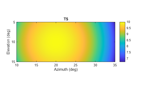
Calculate the reflected sonar signal from a nonfluctuating point target with a peak target strength (TS) of 10.0 db. For illustrative purposes, use a simplified expression for the TS pattern of a target. Real TS patterns are more complicated. The TS pattern covers a range of angles from 10° to 30° in azimuth and from 5° to 15° in elevation. The TS peaks at 20° azimuth and 10° elevation. Assume that the sonar operating frequency is 10 kHz and that the signal is a sinusoid at 9500 kHz.

Create and plot the TS pattern.

azmax = 20.0;
elmax = 10.0;
azpatangs = [10.0:0.1:35.0];
elpatangs = [5.0:0.1:15.0];
tspattern = 10.0*cosd(4*(elpatangs - elmax))'*cosd(4*(azpatangs - azmax));
tspatterndb = 10*log10(tspattern);
imagesc(azpatangs,elpatangs,tspatterndb)
colorbar
axis image
axis tight
title("TS")
xlabel("Azimuth (deg)")
ylabel("Elevation (deg)")

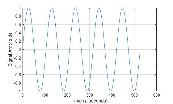
Generate and plot 50 samples of the sonar signal.

freq = 9.5e3;
fs = 100*freq;
nsamp = 500;
t = [0:(nsamp-1)]'/fs;
sig = sin(2*pi*freq*t);
plot(t*1e6,sig)
xlabel("Time (\mu seconds)")
ylabel("Signal Amplitude")
grid

Create the phased.BackscatterSonarTarget System object™.

target = phased.BackscatterSonarTarget(Model="Nonfluctuating", ...
    AzimuthAngles=azpatangs,ElevationAngles=elpatangs, ...
    TSPattern=tspattern);

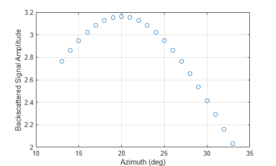
For a sequence of different azimuth incident angles (at constant elevation angle), plot the maximum scattered signal amplitude.

az0 = 13.0;
el = 10.0;
naz = 20;
az = az0 + [0:1:20];
naz = length(az);
ss = zeros(1,naz);
for k = 1:naz
    y = target(sig,[az(k);el]);
    ss(k) = max(abs(y));
end
plot(az,ss,'o')
xlabel('Azimuth (deg)')
ylabel('Backscattered Signal Amplitude')
grid

Backscatter Sonar Signal from Fluctuating Target

Calculate the reflected sonar signal from a Swerling2 fluctuating point target with a peak target strength (TS) of 10.0 db. For illustrative purposes, use a simplified expression for the TS pattern of a target. Real TS patterns are more complicated. The TS pattern covers a range of angles from 10°to 30° in azimuth and from 5° to 15° in elevation. The TS peaks at 20° azimuth and 10° elevation. Assume that the sonar operating frequency is 10 kHz and that the signal is a sinusoid at 9500 kHz.

Create and plot the TS pattern.

azmax = 20.0;
elmax = 10.0;
azpatangs = [10.0:0.1:35.0];
elpatangs = [5.0:0.1:15.0];
tspattern = 10.0*cosd(4*(elpatangs - elmax))'*cosd(4*(azpatangs - azmax));
tspatterndb = 10*log10(tspattern);
imagesc(azpatangs,elpatangs,tspatterndb)
colorbar
axis image
axis tight
title("TS")
xlabel("Azimuth (deg)")
ylabel("Elevation (deg)")

Generate the sonar signal.

freq = 9.5e3;
fs = 10*freq;
nsamp = 50;
t = [0:(nsamp-1)]'/fs;
sig = sin(2*pi*freq*t);

Create the phased.BackscatterSonarTarget System object™.

target = phased.BackscatterSonarTarget(Model="Nonfluctuating", ...
    AzimuthAngles=azpatangs,ElevationAngles=elpatangs, ...
    TSPattern=tspattern,Model="Swerling2");

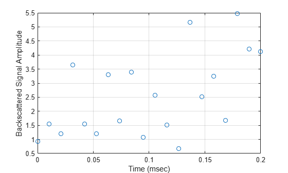
Compute and plot the fluctuating signal amplitude for 20 time steps.

az = 20.0;
el = 10.0;
nsteps = 20;
ss = zeros(1,nsteps);
for k = 1:nsteps
    y = target(sig,[az;el],true);
    ss(k) = max(abs(y));
end
plot([0:(nsteps-1)]*1000/fs,ss,'o')
xlabel("Time (msec)")
ylabel("Backscattered Signal Amplitude")
grid

More About

Backscattered Sound Radiation

For narrowband acoustic signals, the reflected signal, Y, is given by

$$Y=\sqrt{G}\cdot X,$$

where

• X is the incoming signal.

• G is the target gain factor given by 10^TS/10 where TS is the target strength in dB. Specify target strength using the TSPattern property.

For a more detailed explanation of target strength, see [1] [2].

References

[1] Urick, R.J. Principles of Underwater Sound, 3rd Edition. New York: Peninsula Publishing, 1996.

[2] Sherman, C.S., and J. Butler Transducers and Arrays for Underwater Sound. New York: Springer, 2007.

Extended Capabilities

C/C++ Code Generation

Generate C and C++ code using MATLAB® Coder™.

Usage notes and limitations:

See System Objects in MATLAB Code Generation (MATLAB Coder).

Version History

Introduced in R2017a