fitLifetimePDModel

Create specified lifetime PD model object type

Since R2020b

Syntax

pdModel = fitLifetimePDModel(data,ModelType)

pdModel = fitLifetimePDModel(___,Name,Value)

Description

pdModel = fitLifetimePDModel(data,ModelType) creates a lifetime probability of default (PD) model object specified by data and ModelType. fitLifetimePDModel takes in credit data in panel data form and fits a lifetime PD model. ModelType is supported for Logistic, Probit, or Cox.

pdModel = fitLifetimePDModel(___,Name,Value) specifies options using one or more name-value pair arguments in addition to the input arguments in the previous syntax. The available optional name-value pair arguments depend on the specified ModelType.

Examples

Create Logistic Lifetime PD Model

This example shows how to use fitLifetimePDModel to create a Logistic model using credit and macroeconomic data.

Load Data

Load the credit portfolio data.

load RetailCreditPanelData.mat
disp(head(data))

    ID    ScoreGroup    YOB    Default    Year
    __    __________    ___    _______    ____

    1      Low Risk      1        0       1997
    1      Low Risk      2        0       1998
    1      Low Risk      3        0       1999
    1      Low Risk      4        0       2000
    1      Low Risk      5        0       2001
    1      Low Risk      6        0       2002
    1      Low Risk      7        0       2003
    1      Low Risk      8        0       2004

disp(head(dataMacro))

    Year     GDP     Market
    ____    _____    ______

    1997     2.72      7.61
    1998     3.57     26.24
    1999     2.86      18.1
    2000     2.43      3.19
    2001     1.26    -10.51
    2002    -0.59    -22.95
    2003     0.63      2.78
    2004     1.85      9.48

Join the two data components into a single data set.

data = join(data,dataMacro);
disp(head(data))

    ID    ScoreGroup    YOB    Default    Year     GDP     Market
    __    __________    ___    _______    ____    _____    ______

    1      Low Risk      1        0       1997     2.72      7.61
    1      Low Risk      2        0       1998     3.57     26.24
    1      Low Risk      3        0       1999     2.86      18.1
    1      Low Risk      4        0       2000     2.43      3.19
    1      Low Risk      5        0       2001     1.26    -10.51
    1      Low Risk      6        0       2002    -0.59    -22.95
    1      Low Risk      7        0       2003     0.63      2.78
    1      Low Risk      8        0       2004     1.85      9.48

Partition Data

Separate the data into training and test partitions.

nIDs = max(data.ID);
uniqueIDs = unique(data.ID);

rng('default'); % for reproducibility
c = cvpartition(nIDs,'HoldOut',0.4);

TrainIDInd = training(c);
TestIDInd = test(c);

TrainDataInd = ismember(data.ID,uniqueIDs(TrainIDInd));
TestDataInd = ismember(data.ID,uniqueIDs(TestIDInd));

Create Logistic Lifetime PD Model

Use fitLifetimePDModel to create a Logistic model using the training data.

pdModel = fitLifetimePDModel(data(TrainDataInd,:),"Logistic",...
    'AgeVar','YOB',...
    'IDVar','ID',...
    'LoanVars','ScoreGroup',...
    'MacroVars',{'GDP','Market'},...
    'ResponseVar','Default');
disp(pdModel)

  Logistic with properties:

            ModelID: "Logistic"
        Description: ""
    UnderlyingModel: [1x1 classreg.regr.CompactGeneralizedLinearModel]
              IDVar: "ID"
             AgeVar: "YOB"
           LoanVars: "ScoreGroup"
          MacroVars: ["GDP"    "Market"]
        ResponseVar: "Default"
         WeightsVar: ""
       TimeInterval: 1

Display the underlying model.

pdModel.UnderlyingModel

ans = 
Compact generalized linear regression model:
    logit(Default) ~ 1 + ScoreGroup + YOB + GDP + Market
    Distribution = Binomial

Estimated Coefficients:
                               Estimate        SE         tStat       pValue   
                              __________    _________    _______    ___________

    (Intercept)                  -2.7422      0.10136    -27.054     3.408e-161
    ScoreGroup_Medium Risk      -0.68968     0.037286    -18.497     2.1894e-76
    ScoreGroup_Low Risk          -1.2587     0.045451    -27.693    8.4736e-169
    YOB                         -0.30894     0.013587    -22.738    1.8738e-114
    GDP                         -0.11111     0.039673    -2.8006      0.0051008
    Market                    -0.0083659    0.0028358    -2.9502      0.0031761


388097 observations, 388091 error degrees of freedom
Dispersion: 1
Chi^2-statistic vs. constant model: 1.85e+03, p-value = 0

Predict Conditional and Lifetime PD

Use the predict function to predict conditional PD values. The prediction is a row-by-row prediction.

dataCustomer1 = data(1:8,:);
CondPD = predict(pdModel,dataCustomer1)

CondPD = 8×1

    0.0092
    0.0053
    0.0045
    0.0039
    0.0037
    0.0037
    0.0019
    0.0012

Use predictLifetime to predict the lifetime cumulative PD values (computing marginal and survival PD values is also supported). The predictLifetime function uses the ID variable (see the 'IDVar' property for the Logistic object) to transform conditional PDs to cumulative PDs for each ID.

LifetimePD = predictLifetime(pdModel,dataCustomer1)

LifetimePD = 8×1

    0.0092
    0.0145
    0.0189
    0.0228
    0.0264
    0.0300
    0.0319
    0.0330

Validate Model

Use modelDiscrimination to measure the ranking of customers by PD.

DiscMeasure = modelDiscrimination(pdModel,data(TestDataInd,:),DataID='test data');
disp(DiscMeasure)

                            AUROC 
                           _______

    Logistic, test data    0.70009

Use modelDiscriminationPlot to visualize the ROC curve.

modelDiscriminationPlot(pdModel,data(TestDataInd,:),DataID='test data');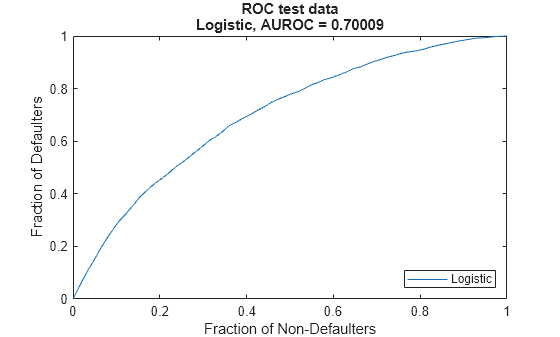

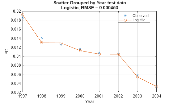
Use modelCalibration to measure the calibration of the predicted PD values. The modelCalibration function requires a grouping variable and compares the accuracy of the observed default rate in the group with the average predicted PD for the group. For example, you can group by calendar year using the 'Year' variable.

CalMeasure = modelCalibration(pdModel,data(TestDataInd,:),'Year',DataID='test data');
disp(CalMeasure)

                                              RMSE  
                                            ________

    Logistic, grouped by Year, test data    0.000453

Use modelCalibrationPlot to visualize the observed default rates compared to the predicted probabilities of default (PD).

modelCalibrationPlot(pdModel,data(TestDataInd,:),'Year',DataID='test data');

Input Arguments

data — Data

table

Data, specified as a table, in panel data form. The data must contain an ID column. The response variable must be a binary variable with the value 0 or 1, with 1 indicating default.

Data Types: table

ModelType — Type of PD model

character vector with value 'Logistic', 'Probit', or 'Cox' | string with value "Logistic", "Probit", or "Cox"

Type of PD model, specified as a scalar string or character vector. Use one of following values:

• Logistic —Fit a Logistic model for lifetime probability. For more information, see Time Interval for Logistic Models.

• Probit — Fit a Probit model for lifetime probability. For more information, see Time Interval for Probit Models.

• Cox — Fit a Cox model for lifetime probability. For more information, see Cox Proportional Hazards Models.

Data Types: string | char

Name-Value Arguments

Specify optional pairs of arguments as Name1=Value1,...,NameN=ValueN, where Name is the argument name and Value is the corresponding value. Name-value arguments must appear after other arguments, but the order of the pairs does not matter.

Before R2021a, use commas to separate each name and value, and enclose Name in quotes.

Example: pdModel = fitLifetimePDModel(data(TrainDataInd,:),ModelType,'AgeVar',"YOB",'IDVar',"ID",'LoanVars',"ScoreGroup",'MacroVars',{'GDP','Market'},'ResponseVar',"Default")

The available name-value pair arguments depend on the value you specify for ModelType.

• Logistic — See Name-Value Arguments.

• Probit — See Name-Value Arguments.

• Cox — See Name-Value Arguments.

Output Arguments

pdModel — Probability of default model

pdModel object

Probability of default model, returned as a pdModel object. Supported classes are Logistic, Probit, or Cox.

References

Independently published

[1] Baesens, Bart, Daniel Roesch, and Harald Scheule. Credit Risk Analytics: Measurement Techniques, Applications, and Examples in SAS. Wiley, 2016.

[2] Bellini, Tiziano. IFRS 9 and CECL Credit Risk Modelling and Validation: A Practical Guide with Examples Worked in R and SAS. San Diego, CA: Elsevier, 2019.

[3] Breeden, Joseph. Living with CECL: The Modeling Dictionary. Santa Fe, NM: Prescient Models LLC, 2018.

[4] Roesch, Daniel and Harald Scheule. Deep Credit Risk: Machine Learning with Python. Independently published, 2020.

Version History

Introduced in R2020b