Overview of Lifetime Probability of Default Models

Regulatory frameworks such as IFRS 9 and CECL require institutions to estimate loss reserves based on a lifetime analysis that is conditional on macroeconomic scenarios. Earlier models were frequently designed to predict one period ahead and often with no explicit sensitivities to macroeconomic scenarios. With the IFRS 9 and CECL regulations, models must predict multiple periods ahead and the models must have an explicit dependency on macroeconomic variables.

The main output of the lifetime credit analysis is the lifetime expected credit loss (ECL). The lifetime ECL consists of the reserves that banks need to set aside for expected losses throughout the life of a loan. There are different approaches to the estimation of lifetime ECL. Some approaches use relatively simple techniques on loss data, with qualitative adjustments. Other approaches use more advanced time-series techniques or econometric models to forecast losses, with dependencies on macro variables. Another methodology uses probability of default (PD) models, loss given default (LGD) models, and exposure at default (EAD) models, and combines their outputs to estimate the ECL. The lifetime PD models in Risk Management Toolbox™ are in the PD-LGD-EAD category.

Traditional PD Models Compared to Lifetime PD Models

Traditional PD models predict the probability of default for the next period (that is, next year, next quarter, and so on). These one-period ahead models include a range of methodologies, such as credit scorecards (creditscorecard), decision trees (fitctree), and transition matrices (transprob). These models include different types of predictors. Some of them are simple, such as customer income, and others are more complex, such as utilization rate, or some other metrics related to the financial activities of the borrower. For these models, the latest observed values of the predictors, possibly with some lagged information, are usually enough to make a prediction, and there is no need to project or forecast the values of the predictors going forward.

In contrast, the lifetime PD models require forward looking values of all predictors to make a prediction of the lifetime PD through the end of the life of the loan. Because the projected values of the predictors are needed, these models can reduce the amount and complexity of predictors and use either predictors with constant values, such as origination score, or predictors that can be projected with little effort, such as loan-to-value ratio. One predictor typically included in these models is the age of the loan. When used for regulatory purposes, macroeconomic predictors must be included in the model, and multiple macroeconomic scenarios are required for the lifetime credit analysis.

Lifetime credit analysis also requires the cumulative lifetime PD, which is a transformation of the predicted, conditional PDs. Specifically, the marginal PD, which is the increments in the cumulative lifetime PD, is used for the computation of the ECL. The survival probability is often reported as well. These alternative versions of the probability are recursive operations on the predicted, conditional PD values for a single loan. In other words, the prediction data may include rows for the same ID a few periods ahead, and the corresponding conditional PDs may show a time-dependent structure. But these conditional PD predictions are "one-period ahead" predictions where the "period" is the same time interval implicit in the training data. Conditional PD predictions are "row-by-row" predictions, where one row of the inputs predicts a conditional PD independently of all other rows. However, for the cumulative lifetime PD, the cumulative PD value for the second period depends on the conditional PDs for the first and second periods, and all subsequent periods have an explicit dependency on the previous period (a recursion). For the lifetime predictions, therefore, the software must know which rows in the inputs correspond to the same loan, so some form of loan identifier is required for the lifetime prediction. Moreover, consecutive rows in the lifetime prediction data must correspond to consecutive time periods, the recursion is defined for consecutive, one-period ahead conditional PDs, it cannot skip periods.

The following table summarizes the differences between traditional PD models and lifetime PD models.

Traditional PD Models	Lifetime PD Models
Predict one period ahead	Predict multiple periods ahead
Predict conditional PD only	Predict conditional PD, cumulative lifetime PD, marginal PD, and survival probability
Predict for each row of the data inputs, independently of all other rows	Predict for all rows of the data inputs that correspond to the same loan; this is a recursive operation that requires some form of loan identifier to know where to start the recursion
Need only most recent observed information to make PD predictions	Need the most recent information and projected, period-by-period values of predictor variables over the lifetime of the loan to make PD predictions
Can use complex predictors that result from nontrivial data processing or data transformations	Typically use simpler predictors, variables that are not hard to project and forecast
Besides loan-specific predictors, models can include macroeconomic variables or an age variable	Besides loan-specific predictors, models must include macroeconomic predictors (especially if used for regulatory purposes) and typically include an age variable

Model Development and Validation

Risk Management Toolbox supports the modeling and validation of lifetime PD models through a family of classes supporting:

• Model fitting with the fitLifetimePDModel

• Prediction of conditional PD with the predict function

• Prediction of lifetime PD (cumulative, marginal, and survival) with the predictLifetime function

• Model discrimination metrics with the modelDiscrimination function

• Plot the ROC curve with the modelDiscriminationPlot function

• Model accuracy (or calibration) metrics with the modelAccuracy function

• Plot observed default rates compared to predicted PDs on grouped data with the modelAccuracyPlot function

The supported model types are Logistic, Probit, Cox, and customLifetimePDModel models.

A typical modeling workflow for lifetime PD analysis includes:

1. Data preparation

   The lifetime PD models require a panel data input for fitting, prediction, and validation. The response variable must be a binary (0 or 1) variable, with 1 indicating default. There is a wide range of tools available to treat missing data (using fillmissing), handle outliers (using filloutliers), and perform other data preparation tasks.

2. Model fitting

   Use the fitLifetimePDModel function to fit a lifetime PD model. You must use the previously prepared data, select a model type, and indicate which variables correspond to loan-specific variables (such as origination score and loan-to-value ratio). Also, you can also include an age variable (such as years on books) and the macroeconomic variables (such as gross domestic product growth or unemployment rate), as well as the ID variable and response variable. You can specify a model description and also specify a model ID or tag for reporting purposes during model validation. Alternatively, you can use customLifetimePDModel to use a function handle to define a custom PD model.

3. Model validation

   There are multiple tasks involved in model validation, including

   • Inspect the underlying statistical model, which is stored in the 'Model' property of the Logistic, Probit, or Cox object. For more information, see Basic Lifetime PD Model Validation.

   • Measure the model discrimination on either training or test data with the modelDiscrimination function. Visualizations can also be generated using the modelDiscriminationPlot function. Data can be segmented to measure discrimination over different segments.

   • Measure the model accuracy (also known as model calibration) on either training or test data with the modelAccuracy function. Visualizations can also be generated using the modelAccuracyPlot function. A grouping variable is required to measure the observed default rate for each group and compare it against the average predicted conditional PD for the group.

   • Validate the model against a benchmark (for example, a champion model). For more information, see Compare Logistic Model for Lifetime PD to Champion Model.

   • Perform a cross-validation analysis to compare alternative models. For more information, see Compare Lifetime PD Models Using Cross-Validation.

   • Perform a qualitative assessment of conditional PD predictions by using the predict function directly with edge cases. Note that model validation relies on the conditional PD predictions generated by the predict function. The predict function is automatically called by modelDiscrimination and modelAccuracy to generate metrics.

   • Visualize the lifetime PD predictions for model validation by using the predictLifetime function with edge cases and then perform a qualitative assessment of the predictions.

Computation of Lifetime ECL

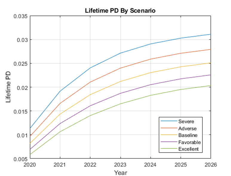
Once you develop and validate a lifetime PD model, you can use it for lifetime ECL analysis. The Expected Credit Loss Computation example demonstrates the basic workflow for computing ECL.

The Expected Credit Loss Computation example shows how to visualize the lifetime PD predictions, for different macro scenarios.

The Expected Credit Loss Computation example also shows how to compute the ECL per scenario and how to compute the final lifetime ECL for a given loan.

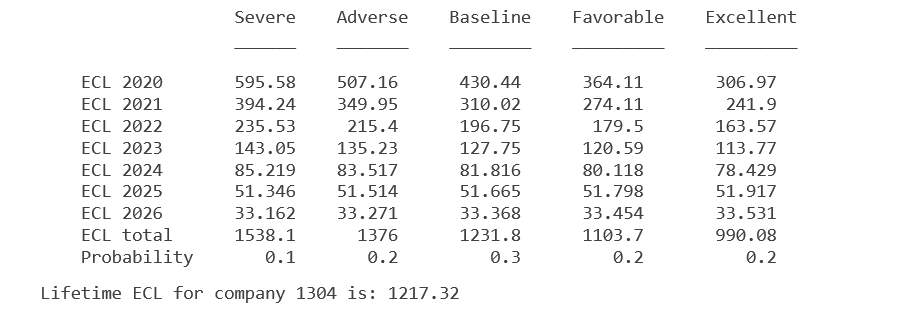
For more information on preparing the data for prediction (including joining loan data projections and macro forecasts) and the additional parameters and computations necessary for the estimation of the lifetime ECL, see Expected Credit Loss Computation and portfolioECL.

Lifetime Credit Analysis Compared to Stress Testing

You can also use the lifetime PD models for stress testing analysis. However, lifetime credit analysis and stress testing have several differences that the following table summarizes.

Stress Testing	Lifetime Credit Analysis
Focus on negative, pessimistic scenarios	Must consider a range of scenarios, including pessimistic, neutral, and optimistic ones
Models are often biased, calibrated to produce more conservative results	Models are expected to be unbiased
Spans a few quarters ahead	Can span many years ahead
Macroeconomic forecasts for stress testing go a few quarters into the future	Macro scenarios reach far into the future and are typically expected to revert to some baseline level after a few quarters

The types of models used for both of these analyses are very similar. You can use lifetime PD models for stress testing analysis with some additional considerations to account for the differences listed in the previous table.

References

[1] Baesens, Bart, Daniel Roesch, and Harald Scheule. Credit Risk Analytics: Measurement Techniques, Applications, and Examples in SAS. Wiley, 2016.

[2] Bellini, Tiziano. IFRS 9 and CECL Credit Risk Modelling and Validation: A Practical Guide with Examples Worked in R and SAS. San Diego, CA: Elsevier, 2019.

[3] Breeden, Joseph. Living with CECL: The Modeling Dictionary. Santa Fe, NM: Prescient Models LLC, 2018.