bsplinepolytraj

Generate polynomial trajectories using B-splines

Since R2019a

Syntax

[q,qd,qdd,pp] = bsplinepolytraj(controlPoints,tInterval,tSamples)

Description

[q,qd,qdd,pp] = bsplinepolytraj(controlPoints,tInterval,tSamples) generates a piecewise cubic B-spline trajectory that falls in the control polygon defined by controlPoints. The trajectory is uniformly sampled between the start and end times given in tInterval. The function returns the positions, velocities, and accelerations at the input time samples, tSamples. The function also returns the piecewise polynomial pp form of the polynomial trajectory with respect to time.

Examples

Compute B-Spline Trajectory for 2-D Planar Motion

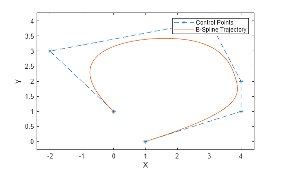
Use the bsplinepolytraj function with a given set of 2-D xy control points. The B-spline uses these control points to create a trajectory inside the polygon. The start and end time for the trajectory are also given.

cpts = [1 4 4 3 -2 0; 0 1 2 4 3 1];
tpts = [0 5];

Compute the B-spline trajectory. The function outputs the trajectory positions (q), velocity (qd), acceleration (qdd), time vector (tvec), and polynomial coefficients (pp) of the polynomial that achieves the waypoints using the control points.

tvec = 0:0.01:5;
[q, qd, qdd, pp] = bsplinepolytraj(cpts,tpts,tvec);

Plot the results. Show the control points and the resulting trajectory inside them.

figure
plot(cpts(1,:),cpts(2,:),'xb-')
hold all
plot(q(1,:), q(2,:))
xlabel('X')
ylabel('Y')
hold off

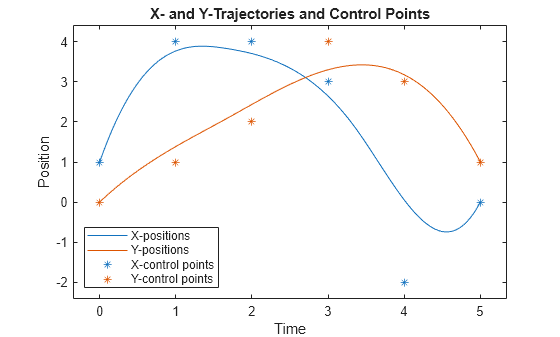
Plot the position of each element of the B-spline trajectory. These trajectories are cubic piecewise polynomials parameterized in time.

figure
plot(tvec,q)
hold all
plot([0:length(cpts)-1],cpts,'x')
xlabel('t')
ylabel('Position Value')
legend('X-positions','Y-positions')
hold off

Interpolate with B-Spline

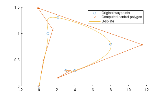
Create waypoints to interpolate with a B-Spline.

wpts1 = [0 1 2.1 8 4 3];
wpts2 = [0 1 1.3 .8 .3 .3];
wpts = [wpts1; wpts2];
L = length(wpts) - 1;

Form matrices used to compute interior points of control polygon

r = zeros(L+1, size(wpts,1));
A = eye(L+1);
for i= 1:(L-1)
    A(i+1,(i):(i+2)) = [1 4 1];
    r(i+1,:) = 6*wpts(:,i+1)';
end

Override end points and choose r0 and rL.

A(2,1:3) = [3/2 7/2 1]; 
A(L,(L-1):(L+1)) = [1 7/2 3/2]; 

r(1,:) = (wpts(:,1) + (wpts(:,2) - wpts(:,1))/2)';
r(end,:) = (wpts(:,end-1) + (wpts(:,end) - wpts(:,end-1))/2)';

dInterior = (A\r)';

Construct a complete control polygon and use bsplinepolytraj to compute a polynomial with the new control points

cpts = [wpts(:,1) dInterior wpts(:,end)];
t = 0:0.01:1;
q = bsplinepolytraj(cpts, [0 1], t);

Plot the results. Show the original waypoints, the computed polygon, and the interpolated B-spline.

figure;
hold all
plot(wpts1, wpts2, 'o');
plot(cpts(1,:), cpts(2,:), 'x-');
plot(q(1,:), q(2,:));
legend('Original waypoints', 'Computed control polygon', 'B-spline');

[1] Farin, Section 9.1

Input Arguments

controlPoints — Points for control polygon

n-by-p matrix

Points for control polygon of B-spline trajectory, specified as an n-by-p matrix, where n is the dimension of the trajectory and p is the number of control points.

Example: [1 4 4 3 -2 0; 0 1 2 4 3 1]

Data Types: single | double

tInterval — Start and end times for trajectory

two-element vector

Start and end times for the trajectory, specified as a two-element vector.

Example: [0 10]

Data Types: single | double

tSamples — Time samples for trajectory

vector

Time samples for the trajectory, specified as a vector. The output position, q, velocity, qd, and accelerations, qdd, are sampled at these time intervals.

Example: 0:0.01:10

Data Types: single | double

Output Arguments

q — Positions of trajectory

vector

Positions of the trajectory at the given time samples in tSamples, returned as a vector.

Data Types: single | double

qd — Velocities of trajectory

vector

Velocities of the trajectory at the given time samples in tSamples, returned as a vector.

Data Types: single | double

qdd — Accelerations of trajectory

vector

Accelerations of the trajectory at the given time samples in tSamples, returned as a vector.

Data Types: single | double

pp — Piecewise-polynomial

structure

Piecewise-polynomial, returned as a structure that defines the polynomial for each section of the piecewise trajectory. You can build your own piecewise polynomials using mkpp, or evaluate the polynomial at specified times using ppval. The structure contains the fields:

• form: 'pp'.

• breaks: p-element vector of times when the piecewise trajectory changes forms. p is the number of waypoints.

• coefs: n(p–1)-by-order matrix for the coefficients for the polynomials. n(p–1) is the dimension of the trajectory times the number of pieces. Each set of n rows defines the coefficients for the polynomial that described each variable trajectory.

• pieces: p–1. The number of breaks minus 1.

• order: Degree of the polynomial + 1. For example, cubic polynomials have an order of 4.

• dim: n. The dimension of the control point positions.

References

[1] Farin, Gerald E. Curves and Surfaces for Computer Aided Geometric Design: A Practical Guide. San Diego, CA: Academic Press, 1993.

Extended Capabilities

C/C++ Code Generation
Generate C and C++ code using MATLAB® Coder™.

Version History

Introduced in R2019a