Frequency-Response Analysis of MIMO System

R2026b

This example shows how to estimate and analyze the multi-input/multi-output (MIMO) transfer function for a two-body oscillator. To estimate transfer functions and perform modal analysis, you can use these Signal Processing Toolbox™ functions:

• tfestimate — Transfer function estimate

• modalfrf — Frequency-response functions for modal analysis

• modalsd — Generate stabilization diagram for modal analysis

• modalfit — Modal parameters from frequency-response functions

This example computes the time-domain model by calculating the inputs and outputs that emulate measurements of the two-body oscillating system. Then, the example performs these analysis:

• Theoretical Frequency Response — Use the Z-transform definition to calculate the frequency-domain transfer function of the system.

• Transfer Function Estimate Using tfestimate — Use tfestimate to estimate the MIMO transfer-function frequency response from the simulated measurement data.

• Transfer Function Estimate Using Modal Analysis — Use modalfrf, modalsd, and modalfit to obtain frequency-response functions and analyze the MIMO system.

The comparison between the outputs of these analysis functions shows how you can retrieve the transfer function from system input/output data.

Two-Body Oscillating System

An ideal one-dimensional discrete-time oscillating system consists of two masses, $m_1$ and $m_2$, confined between two walls. The units are such that $m_1=1$ kg and $m_2=\mu$ kg. Each mass is attached to the nearest wall by a spring with elastic constant $k$ (in N/m). An identical spring connects the two masses. Three dampers impede the motion of the masses by exerting on them forces proportional to speed, with damping constant $b$ (in kg/s). Two sensors sample $r_1$ and $r_2$ (in $m$), the displacements of the masses, at a rate $F_s$.

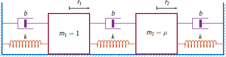
The system can be described by the state-space model

$$\begin{array}{c}x(k+1)=Ax(k)+Bu(k),\\ y(k)=Cx(k)+Du(k),\end{array}$$

where $$x={\left[\begin{array}{cccc}{r}_1& v_1& r_2& v_2\end{array}\right]}^T$$ is the state vector, $$r_i$$ and $$v_i$$ are respectively the location and the velocity of the $$i$$th mass, $$u={\left[\begin{array}{cc}{u}_1& u_2\end{array}\right]}^T$$ is the vector of input driving forces, and $$y={\left[\begin{array}{cc}{r}_1& r_2\end{array}\right]}^T$$ is the output vector. The state-space matrices in discrete time are

$$A_d=\exp \left(\frac{1}{F_s}{A}_c\right),B_d=A_c^{-1}(A-I)B_c,C_d=\left[\begin{array}{cccc}1& 0& 0& 0\\ 0& 0& 1& 0\end{array}\right],D_d=\left[\begin{array}{cc}0& 0\\ 0& 0\end{array}\right],$$

$I$ is the $4\times 4$ identity matrix, and the continuous-time state-space matrices are

$$A_c=\left[\begin{array}{cccc}0& 1& 0& 0\\ -2k& -2b& k& b\\ 0& 0& 0& 1\\ k/\mu & b/\mu & -2k/\mu & -2b/\mu \end{array}\right],B_c=\left[\begin{array}{cc}0& 0\\ 1& 0\\ 0& 0\\ 0& 1/\mu \end{array}\right].$$

Time-Domain Model

Generate 24,000 time samples, equivalent to 10 minutes at a sample rate of 40 Hz.

Fs = 40;
N = 24000;
t = 1/Fs*(0:N-1);

Generate the state-space model for a two-body oscillating system. Set $k=400$ N/m, $b=0.1$ kg/s, and $\mu =0.1$.

k = 400;
b = 0.1;
mu = 0.1;
Ac = [0 1 0 0;-2*k -2*b k b;0 0 0 1;k/mu b/mu -2*k/mu -2*b/mu];
Bc = [0 0;1 0;0 0;0 1/mu];

Ad = expm(Ac/Fs);
Bd = Ac\(Ad-eye(4))*Bc;
Cd = [1 0 0 0;0 0 1 0];
Dd = zeros(2);

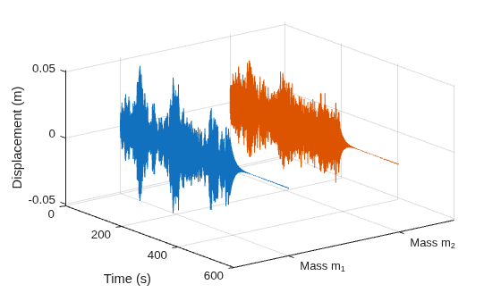
A random input drives the masses for the first 390 seconds and then the masses are left to rest. Set the initial conditions of location and velocity to zero. Use the state-space model to compute the time evolution of the system. Plot the displacements of the masses as a function of time.

u = randn(2,N);
u(:,t>390) = 0;

y = zeros(2,1);
x = zeros(4,1);
for iter = 1:N
    y(:,iter) = Cd*x + Dd*u(:,iter);
    x = Ad*x + Bd*u(:,iter);
end

Set the system time, input, and response data to vertical vector format.

t = t.';
u = u.';
y = y.';

Plot the system response over time for the two masses.

plot3([1 2].*ones(size(t)),t,y)
set(gca,Ydir="reverse")
xticks([1 2])
xticklabels("Mass m_" + [1 2])
ylabel("Time (s)")
zlabel("Displacement (m)")
xlim([0.5 2.5])
grid on

To save the system data, uncomment this line.

% save MIMOdata

Theoretical Frequency Response

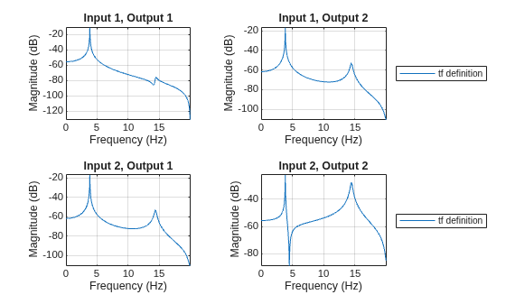
The frequency-response function of a discrete-time system is the Fourier transform of its time-domain transfer function or, equivalently, the Z-transform of the transfer function evaluated at the unit circle.

Compute the theoretical frequency-response functions. Use 2048 frequency points to evaluate the responses.

[b1,a1] = ss2tf(Ad,Bd,Cd,Dd,1);
[b2,a2] = ss2tf(Ad,Bd,Cd,Dd,2);

nfft = 2048;
fz = (0:nfft-1)/nfft*Fs/2;
ztf(1,:,1) = freqz(b1(1,:),a1,fz,Fs);
ztf(1,:,2) = freqz(b1(2,:),a1,fz,Fs);
ztf(2,:,1) = freqz(b2(1,:),a2,fz,Fs);
ztf(2,:,2) = freqz(b2(2,:),a2,fz,Fs);

Plot the theoretical frequency-response functions. The hPlotComparison helper function is at the end of this example.

hPlotComparison(fz,ztf)

Transfer Function Estimate Using tfestimate

Use the system data and the tfestimate function without output arguments to plot the estimate of the MIMO transfer functions. Select the "mimo" option to produce all four transfer functions. Use a periodic 5000-sample Hann window to divide the signals into segments. Specify 2500 samples of overlap between adjoining segments. Store the transfer function of the system as a function of frequency.

wind = hann(5000,"periodic");
nov = 2500;

[tXY,ft] = tfestimate(u,y,wind,nov,nfft,Fs,"mimo");

Verify that the estimate computed by tfestimate coincides with the definition.

hPlotComparison(fz,ztf,ft,tXY,"tfestimate")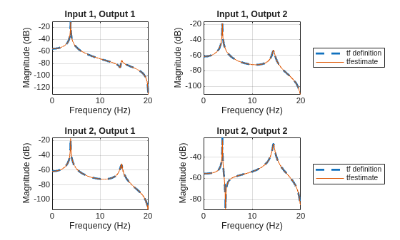

Transfer Function Estimate Using Modal Analysis

Estimate the modal frequency response function of the system using the modalfrf function. Specify the sensor data type as measured displacements.

[frf,f] = modalfrf(u,y,Fs,wind,nov,Sensor="dis");

Plot the estimates and overlay the theoretical predictions.

hPlotComparison(fz,ztf,f,frf,"modalfrf")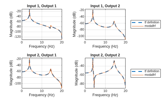

Use modalsd with no output arguments to generate a stabilization diagram for modal analysis and estimate the minimum number of modes. Use a maximum of 10 modes and pick the least-squares rational function estimation method for the calculation.

figure
modalsd(frf,f,Fs,MaxModes=10,FitMethod="lsrf")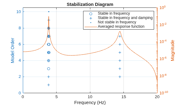

The stabilization diagram shows two "+" marks for 2, 4, 5 and higher model order, indicating a stable modal fit for both frequency and damping using at least two modes.

Estimate the natural frequencies, damping ratios, and mode shapes of the system. Use the modalfit function with two modes and pick the least-squares rational function estimation method for the calculation. Obtain the reconstructed transfer functions of the system in the frequency domain.

nModes = 2;
[fn,dr,ms,ofrf] = modalfit(frf,f,Fs,nModes,FitMethod="lsrf");

Compare the natural frequencies to the theoretical predictions for an undamped system.

fn_theo = sqrt(eig([2*k -k;-k/mu 2*k/mu]))/(2*pi);
disp(table(fn,fn_theo,dr,RowNames= "Mode " + (1:nModes)', ...
    VariableNames=["fn" "fn_theo" "dr"]))

                fn      fn_theo       dr    
              ______    _______    _________

    Mode 1    3.8476     3.847     0.0035235
    Mode 2    3.8566    14.426     0.0010752

The proximity in value of the damping ratio (dr) to zero indicates an underdamped system. The natural frequencies of the system (fn) approach the equivalent undamped natural frequency (fn_theo).

Compare the transfer-function definition with the recovered transfer function from the output of modalfit.

hPlotComparison(fz,ztf,f,ofrf,"modalfit")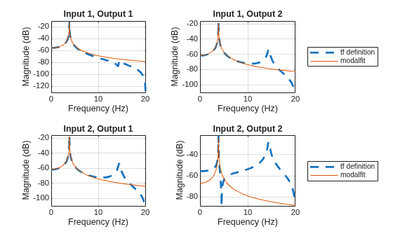

The natural frequencies agree between the recovered and theoretical frequency-response functions despite the differences outside the natural frequencies, correlating with the two modes calculated with modalfit.

Comparison

Compare all transfer function estimation methods discussed in this example.

hPlotComparison(fz,ztf,ft,tXY,"tfestimate", ...
    f,frf,"modalfrf",f,ofrf,"modalfit")

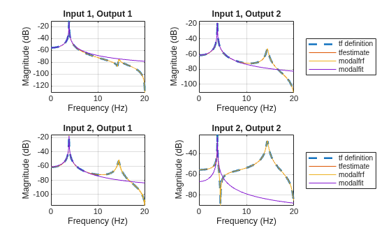
This example uses the tfestimate, modalfrf, modalsd, and modalfit functions to perform frequency-response analysis based on the space-state model of a mass-spring-damper oscillator MIMO system. The functions tfestimate and modalfrf estimate and plot the frequency response of the system, given the information about the system input and output in the time domain. The function modalsd helps to identify the number of modes to use for modal fit. The modal parameters calculated using the function modalfit also help retrieve the frequency response of the system.

Appendix: Helper Function

The hPlotComparison function plots and formats a comparison between theoretical and estimated transfer functions.

function hPlotComparison(varargin)
tiledlayout("flow")
for jk = 1:2
    for kj = 1:2
        nexttile
        if nargin==2
            plot(varargin{1},mag2db(abs(varargin{2}(jk,:,kj))))
        else
            plot(varargin{1}, ...
                mag2db(abs(varargin{2}(jk,:,kj))),"--",LineWidth=2)
        end
        hold on
        for it = 1:fix(nargin/3)
            plot(varargin{3*it},mag2db(abs(varargin{3*it+1}(:,jk,kj))))
        end
        hold off
        grid on
        axis tight
        title("Input " + jk + ", Output " + kj)
        xlabel("Frequency (Hz)")
        ylabel("Magnitude (dB)")
    end
    legend("tf definition",varargin{5:3:end},Location="eastoutside")
end
end