NLMEResults

Results object containing estimation results from nonlinear mixed-effects modeling

Description

The NLMEResults object contains estimation results from fitting a nonlinear mixed-effects model using sbiofitmixed.

Creation

Use the sbiofitmixed function to create an NLMEResults object.

Properties

FixedEffects — Estimates, standard errors, and relative standard errors for fixed effects

table

Estimates, standard errors, and relative standard errors (RSE) for fixed effects, specified as a table.

An RSE is a measure of the precision of a given estimated value. The value range is [0, Inf]. A value closer to 0 indicates greater precision of the estimate. For details, see RSE.

RandomEffects — Estimated random effects for each group

table

Estimated random effects for each group, specified as a table.

IndividualParameterEstimates — Estimated parameter values, including fixed and random effects

table

Estimated parameter values, including fixed and random effects, specified as a table.

PopulationParameterEstimates — Estimated parameter values, including only fixed effects

table

Estimated parameter values, including only fixed effects, specified as a table.

RandomEffectCovarianceMatrix — Covariance matrix of random effects

table

Covariance matrix of random effects, specified as a table.

stats — Statistics returned by the nlmefit and nlmefitsa algorithm

structure array

Statistics returned by the nlmefit (Statistics and Machine Learning Toolbox) and nlmefitsa (Statistics and Machine Learning Toolbox) algorithm, specified as a structure array.

CovariateNames — Covariate names

cell array of character vectors

Covariate names, specified as a cell array of character vectors.

LogLikelihood — Maximized loglikelihood for fitted model

scalar

Maximized loglikelihood for the fitted model, specified as a scalar.

AIC — Akaike Information Criterion (AIC)

scalar

Akaike Information Criterion (AIC), specified as a scalar. The AIC is calculated as AIC = 2*(-LogLikelihood + P), where P is the number of parameters. For details, see nlmefit (Statistics and Machine Learning Toolbox).

BIC — Bayes Information Criterion (BIC)

scalar

Bayes Information Criterion (BIC), specified as a scalar. The BIC is calculated as BIC = -2*LogLikelihood + P*log(N), where N is the number of observations or groups, and P is the number of parameters. For details, see nlmefit (Statistics and Machine Learning Toolbox).

DFE — Degrees of freedom for error

scalar

Degrees of freedom for error (DFE), specified as a scalar. The DFE is calculated as DFE = N-P, where N is the number of observations and P is the number of parameters.

ParameterVariability — Parameter estimate variability and quality

table

Parameter estimate variability and quality, specified as a table.

The table contains the following variables for each parameter estimate:

• CV — Coefficient of variation (%CV) that measures the inter-individual variability of a parameter using the estimated fixed and random effects [2]. The value range is [0,Inf]. A value closer to 0 indicates less variability in the parameter across individuals. The software calculates %CV for parameters for which the metric can be computed analytically, that is, for parameters that have:

  • a random effect

  • log transformation or no parameter transformation

  • no covariates

  If the parameter is not supported, the software reports the value of CV as NaN. For details, see Coefficient of Variation (%CV).

• Shrinkage — Eta-shrinkage that represents the shrinkage of random effects (etas). The value range is [-Inf,1]. A positive shrinkage value closer to 0 indicates that the model has better captured individual parameter estimates. A negative value suggests model misspecification [3]. The software reports Shrinkage for any parameter with a random effect. If the parameter is not supported, the software reports the value of Shrinkage as NaN. For details, see Shrinkage.

If a parameter does not have a random effect, it does not appear in the ParameterVariability table.

EpsilonShrinkage — Shrinkage of individual weighted residuals

scalar

Shrinkage of individually-weighted residuals (IWRES), returned as a scalar. The value range is [-Inf,1]. A positive shrinkage value closer to 0 indicates that the model has better captured individual parameter estimates. A negative value suggests model misspecification [3]. The software calculates and reports EpsilonShrinkage as a single value for the entire fit using the IWRES values for all responses. For details, see Shrinkage.

Data — Data used for fitting

groupedData object

Data used for fitting, specified as a groupedData object.

This Data property contains a copy of groupedData specified as the input data in the sbiofitmixed call or the Data property of a fitproblem object.

EstimatedParameterNames — Estimated parameter names

cell array of character vectors

Estimated parameter names, specified as a cell array of character vectors.

ErrorModelInfo — Table describing the error models and estimated error model parameters

table

Table describing the error models and estimated error model parameters, specified as a table.

The table has one row with three variables: ErrorModel, a, and b. The ErrorModel variable is categorical. The variables a and b can be NaN when they do not apply to a particular error model.

There are four built-in error models. Each model defines the error using a standard mean-zero and unit-variance (Gaussian) variable e, the function value f, and one or two parameters a and b. In SimBiology^®, the function f represents simulation results from a SimBiology model.

• 'constant': $$y=f+ae$$

• 'proportional': $$y=f+b\left|f\right|e$$

• 'combined': $$y=f+(a+b\left|f\right|)e$$

• 'exponential': $$y=f\ast \exp (ae)$$

EstimationFunction — Name of the estimation function

'nlmefit' | 'nlmefitsa'

Name of the estimation function, specified as 'nlmefit' or 'nlmefitsa'.

Note

If you are using the nlmefitsa method, Loglikelihood, AIC, BIC, and RSE are empty by default. To calculate these values, specify the loglikelihood approximation method LogLikMethod (Statistics and Machine Learning Toolbox) as an option. For example, to use the linearization as the loglikelihood approximation method, specify:

opt.LogLikMethod = "lin";

For details on how to set up the options for fitproblem, see Options. For sbiofitmixed, see opt.

Object Functions

boxplot	Create box plot showing the variation of estimated SimBiology model parameters
covariateModel	Return a copy of the covariate model that was used for the nonlinear mixed-effects estimation using sbiofitmixed
fitted	Return the simulation results of a fitted nonlinear mixed-effects model
plot	Compare simulation results to the training data, creating a time-course subplot for each group
plotActualVersusPredicted	Compare predictions to actual data, creating a subplot for each response
plotParameterStats	Show box plot, violin plot, and swarm scatter plots for parameter estimates
plotResidualDistribution	Plot the distribution of the residuals
plotResiduals	Plot the residuals for each response, using the time, group, or prediction as the x-axis
predict	Simulate and evaluate fitted SimBiology model
random	Simulate a SimBiology model, adding variations by sampling the error model
summary	Return parameter estimates and fit quality statistics from SimBiology nonlinear mixed-effects estimation

Examples

Fit One-Compartment PK Model to Phenobarbital Data

This example uses data collected on 59 preterm infants given phenobarbital during the first 16 days after birth [1]. Each infant received an initial dose followed by one or more sustaining doses by intravenous bolus administration. A total of between 1 and 6 concentration measurements were obtained from each infant at times other than dose times, for a total of 155 measurements. Infant weights and APGAR scores (a measure of newborn health) were also recorded.

Load the data.

load pheno.mat ds

Convert the dataset to a groupedData object, a container for holding tabular data that is divided into groups. It can automatically identify commonly used variable names as the grouping variable or independent (time) variable. Display the properties of the data and confirm that GroupVariableName and IndependentVariableName are correctly identified as 'ID' and 'TIME', respectively.

data = groupedData(ds);
data.Properties

ans = struct with fields:
                Description: ''
                   UserData: []
             DimensionNames: {'Observations'  'Variables'}
              VariableNames: {'ID'  'TIME'  'DOSE'  'WEIGHT'  'APGAR'  'CONC'}
              VariableTypes: ["double"    "double"    "double"    "double"    "double"    "double"]
       VariableDescriptions: {}
              VariableUnits: {}
         VariableContinuity: []
                   RowNames: {}
           CustomProperties: [1×1 matlab.tabular.CustomProperties]
          GroupVariableName: 'ID'
    IndependentVariableName: 'TIME'

Create a simple one-compartment PK model with bolus dosing and linear clearance to fit such data. Use the PKModelDesign object to construct the model. Each compartment is defined by a name, dosing type, a clearance type, and whether or not the dosing requires a lag parameter. After constructing the model, you can also get a PKModelMap object map that lists the names of species and parameters in the model that are most relevant for fitting.

pkmd = PKModelDesign;
addCompartment(pkmd,'Central','DosingType','Bolus',...
                    'EliminationType','linear-clearance',...
                    'HasResponseVariable',true,'HasLag',false);
[onecomp, map] = pkmd.construct;

Describe the experimentally measured response by mapping the appropriate model component to the response variable. In other words, indicate which species in the model corresponds to which response variable in the data. The PKModelMap property Observed indicates that the relevant species in the model is Drug_Central, which represents the drug concentration in the system. The relevant data variable is CONC, which you visualized previously.

map.Observed

ans = 1×1 cell array
    {'Drug_Central'}

Map the Drug_Central species to the CONC variable.

responseMap = 'Drug_Central = CONC';

The parameters to estimate in this model are the volume of the central compartment Central and the clearance rate Cl_Central. The PKModelMap property Estimated lists these relevant parameters. The underlying algorithm of sbiofitmixed assumes parameters are normally distributed, but this assumption may not be true for biological parameters that are constrained to be positive, such as volume and clearance. Specify a log transform for the estimated parameters so that the transformed parameters follow a normal distribution. Use an estimatedInfo object to define such transforms and initial values (optional).

map.Estimated

ans = 2×1 cell
    {'Central'   }
    {'Cl_Central'}

Define such estimated parameters, appropriate transformations, and initial values.

estimatedParams = estimatedInfo({'log(Central)','log(Cl_Central)'},'InitialValue',[1 1]);

Each infant received a different schedule of dosing. The amount of drug is listed in the data variable DOSE. To specify this dosing during fitting, create dose objects from the data. These objects use the property TargetName to specify which species in the model receives the dose. In this example, the target species is Drug_Central, as listed by the PKModelMap property Dosed.

map.Dosed

ans = 1×1 cell array
    {'Drug_Central'}

Create a sample dose with this target name and then use the createDoses method of groupedData object data to generate doses for each infant based on the dosing data DOSE.

sampleDose = sbiodose('sample','TargetName','Drug_Central');
doses = createDoses(data,'DOSE','',sampleDose);

Fit the model.

[nlmeResults,simI,simP] = sbiofitmixed(onecomp,data,responseMap,estimatedParams,doses,'nlmefit');

Visualize the fitted results using individual-specific parameter estimates.

plot(nlmeResults,'ParameterType','individual');

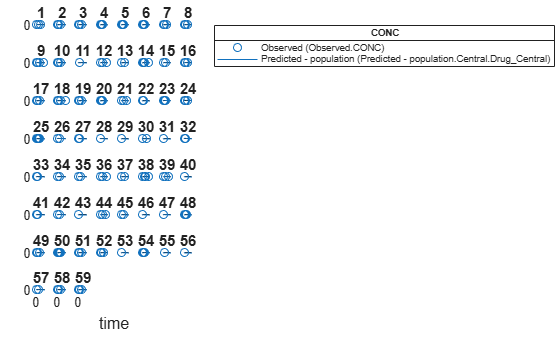
Visualize the fitted results using population parameter estimates.

plot(nlmeResults,'ParameterType','population');

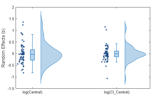
Display the statistics of parameter estimates using box plots, swarm scatter plots, and violin plots.

plotParameterStats(nlmeResults,"box","violin","swarm");

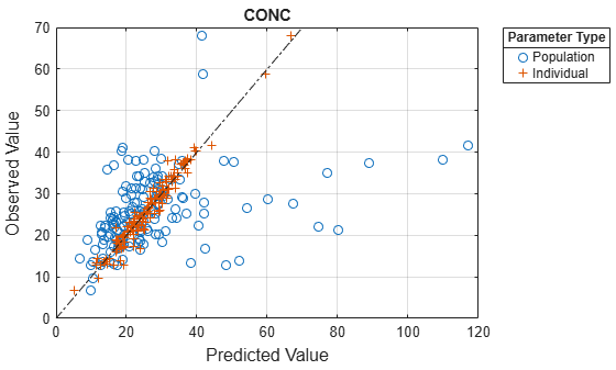
Compare the model predictions to the actual data.

plotActualVersusPredicted(nlmeResults);

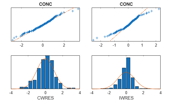
Plot the distribution of residuals.

plotResidualDistribution(nlmeResults);

Plot residuals for each response using the model predictions on x-axis.

plotResiduals(nlmeResults,'Predictions');

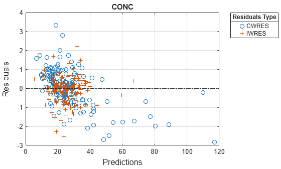
Get the summary of the fit results.

stats.Name contains the name for each table from stats.Table, which contains a list of tables with estimated parameter values and fit quality statistics.

fitMetrics = summary(nlmeResults);

Display the table that contains individual estimates summary statistics.

tableToShow = "Individual Estimates Summary Statistics";
tableNames = {fitMetrics.Name};
tfShowTable = matches(tableNames,tableToShow);
disp(fitMetrics(tfShowTable).Table);

          Statistic           Central    Cl_Central
    ______________________    _______    __________

    {'Minimum'           }    0.62029    0.0021127 
    {'Lower Quartile'    }     1.0676     0.005365 
    {'Median'            }     1.3725    0.0061236 
    {'Upper Quartile'    }     1.6717    0.0068616 
    {'Maximum'           }     5.4555     0.019276 
    {'Mean'              }     1.5713    0.0064928 
    {'Standard Deviation'}    0.90279    0.0026232 

More About

RSE

An RSE is a measure of the precision of a given estimated value. The general formula is:

$$\text{RSE=100}\times \frac{\text{SE}\left(\widehat{\theta }\right)}{\left|\widehat{\theta }\right|},$$

where $$\widehat{\theta }$$ is the estimated value and SE($$\widehat{\theta }$$) is the estimated standard deviation of a given fixed effect.

SimBiology computes the ith fixed effect of a NLMEResults object results as follows:

$${\text{RES}}_{\text{i}}=100\times \frac{\text{results}\text{.FixedEffects}\text{.StandardError(i)}}{\left|\text{results}\text{.FixedEffects}\text{.Estimate(i)}\right|}.$$

Coefficient of Variation (%CV)

A coefficient of variation (%CV) measures the inter-individual variability of a parameter using the estimated fixed and random effects [2]. The general formula is:

$$\text{\%CV=100}\times \frac{{\text{σ}}_{\text{estimate}}}{{\text{μ}}_{\text{estimate}}},$$

where $${\sigma }_{estimate}$$ is the standard deviation of the estimate. $${\mu }_{estimate}$$ is the mean of untransformed parameter given the variance of the random effect eta (η) and the fixed effect estimates thetas (θs).

SimBiology reports %CV only when it can be computed analytically from the estimated fixed and random effects. Specifically, to calculate $${\sigma }_{estimate}$$ and $${\mu }_{estimate}$$, consider the untransformed parameter as a function of a random variable η (with mean=0 and variance = $${\sigma }_{\eta }^2$$) and thetas.

• If the parameter P has no parameter transformation or covariates, that is, P = theta1+eta1, then:

  • $${\sigma }_P^2={\sigma }_{{\eta }_1}^2$$ because theta1 is fixed.

  • $${\mu }_P={\theta }_1$$ because theta1 is constant and $${\mu }_{{\eta }_1}=0$$.

• If the parameter P is log-transformed, that is, P = exp(theta1+eta1), then $$\text{\%CV=100}\times \sqrt{{\text{e}}^{{\text{σ}}_{{\text{η}}_{\text{1}}}^{\text{2}}}\text{-1}}$$.

Shrinkage

A shrinkage value represents the quality of individual estimates and the extent to which these estimates "shrink" towards the population mean due to insufficient information in the data to estimate the random effects precisely.

Theoretically, a shrinkage value can be negative if there are rich data with a small number of subjects or when parameter variance is fixed to a lower value than the true value . Negative shrinkage suggests model misspecification [3]. There are two shrinkage metrics: Eta-shrinkage and Epsilon-shrinkage.

Eta-shrinkage measures how closely standard deviation of the estimated random effects (etas) matches the estimated standard deviation of etas. The general formula is:

$${\text{η}}_{\text{shrinkage}}\text{=1}-\frac{\text{σ}\left({\text{η}}_{\text{EBE}}\right)}{{\text{σ}}_{\text{η}}},$$

where $${\eta }_{EBE}$$ is the empirical Bayes estimates of the random effects for each individual and $${\sigma }_{\eta }$$ is the estimated standard deviation from the covariance matrix for the random effects [3]. SimBiology computes the eta-shrikage of an NLMEResults object results as follows:

$${\text{η}}_{{}_{\text{shrinkage}}}^{\text{i}}\text{=1}-\frac{\text{std}\left(\text{results}\text{.RandomEffects}\text{.Estimate(i,:)}\right)}{\sqrt{\text{results}\text{.RandomEffectCovarianceMatrix(i,i)}}}.$$

Epsilon-shrinkage represents the shrinkage of individually-weighted residuals (IWRES) which is assumed to have unit variance for informative data, but shrinks to zero variance due to overfitting for insufficient data [3]. The general formula is:

$${\text{ε}}_{\text{shrinkage}}\text{=1}-\text{σ}\left(\text{IWRES}\right)\text{.}$$

SimBiology computes the epsilon-shrinkage as follows:

$${\epsilon }_{shrinkage}\text{=1}-\text{std(results}\text{.stats}\text{.iwres(:))}\text{.}$$

References

[1] Grasela T.H. Jr, and Donn S.M. "Neonatal population pharmacokinetics of phenobarbital derived from routine clinical data." Developmental Pharmacology and Therapeutics 8, no. 6 (1985): 374–83. https://doi.org/10.1159/000457062.

[2] Mould, D.R., and Upton, R.N. “Basic Concepts in Population Modeling, Simulation, and Model‐Based Drug Development—Part 2: Introduction to Pharmacokinetic Modeling Methods.” CPT: Pharmacometrics & Systems Pharmacology 2, no. 4 (2013): 1–14. https://doi.org/10.1038/psp.2013.14.

[3] Savic, Radojka M., and Mats O. Karlsson. “Importance of Shrinkage in Empirical Bayes Estimates for Diagnostics: Problems and Solutions.” The AAPS Journal 11, no. 3 (2009): 558–69.https://doi.org/10.1208/s12248-009-9133-0.

Version History

Introduced in R2014a

R2026a: Access fit quality metrics for nonlinear mixed-effects (NLME) estimates

You can now access the following metrics for your NLME fit results:

• Relative standard error (RSE) for checking the precision of population estimates. For details, see FixedEffects.

• Coefficient of variation (%CV) for assessing the variability among individuals. For details, see ParameterVariability.

• Shrinkage information for assessing the quality of individual estimates. You can access both η-shrinkage for each random effect and ε-shrinkage as a single value per fit, where the fit uses individually-weighted residual values (IWRES). For details, see ParameterVariability and EpsilonShrinkage.