Nonlinearities and Noise in Idealized Baseband Amplifier Block
Use the Idealized Baseband Amplifier block to simulate nonlinearities and noise in your RF system design. The Amplifier block provides four nonlinearity models and three options to represent noise.
Nonlinearity Models in Idealized Amplifier Block
Cubic Polynomial
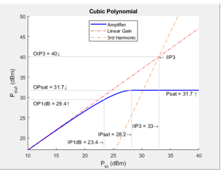
The Cubic polynomial model uses linear power gain to determine the linear coefficient of a third-order polynomial and either IP3, P1dB, or Psat to determine the third - order coefficient of the polynomial. The general form of cubic nonlinearity models the AM/AM characteristics as
where FAM/AM(|u|) is the
magnitude of the output signal, |u| is the magnitude of the input
signal, c1 is the coefficient of the
linear gain term, and c3 is the
coefficient of the cubic gain term. The results for IIP3, OIP3, IP1dB, OP1dB, IPsat
and OPsat are taken from [1]. The coefficient
c3 are given in this
table.
| Nonlinearity Type | Equations |
|---|---|
| Input third-order intercept point, IIP3 (dBm) | IIP3 is given in dBm. |
| Output third-order intercept point,OIP3 (dBm) | OIP3 is given in dBm. |
| Input 1 dB gain compression power,IP1dB (dBm) | IP1dB is given in dBm. |
| Output 1 dB gain compression power, OP1dB (dBm) | OP1dB is given in dBm, and LGdB is the linear gain in dB. |
| Input saturation power, IPsat (dBm) | IPsat is given in dBm. |
| Output saturation power, OPsat (dBm) | OPsat is given in dBm. |
AM/AM-AM/PM
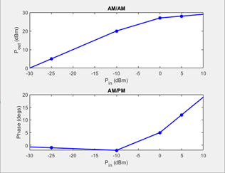
The AM/AM-AM/PM model uses a lookup table to specify the amplifier power characteristics. The table returns interpolated or extrapolated values using linear interpolation. Each row in the table expresses the relationship between output power or phase change as a function of input power.
where uout is the output signal and u is the magnitude of input signal.
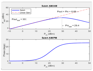
Saleh
The Saleh model is based on normalized transfer function. Use the input / output scaling parameters to adjust signal levels from their normalized values. For Saleh, the AM/AM parameters alphaAM/AM and betaAM/AM are used to compute the amplitude gain for an input signal using the following equation:
where |u| is the magnitude of the scaled signal and u is calculated as:
For Saleh, the AM/PM parameters alphaAM/PM and betaAM/PM are used to compute the phase change for an input signal using the following equation:
where |u| is the magnitude of the scaled signal and angle is a MATLAB® function that returns the phase angle of u.
The scaled output signal, uout is calculated as:
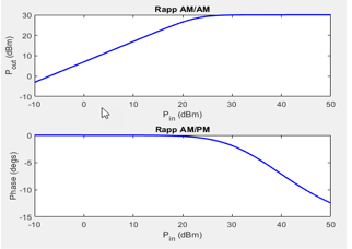
Modified Rapp
The Modified Rapp model is based on normalized transfer functions.
Use the input and output scaling parameters to adjust the signal levels from their
normalized values.
The AM/AM characteristics for Modified Rapp are given
by:
where |u| is the magnitude of input signal, glin is 10(Linear Gain (dB)/20), and is the amplitude gain of the amplifier, Vsat is Output saturation level (V), and p is Magnitude smoothness factor.
The AM/PM characteristics for Modified Rapp is given by:
where u is the input signal, A is the Phase gain
(rad), B is Phase
saturation, q1 and
q2 are Phase smoothness
factor and angle is a MATLAB function which
returns phase angle of u.
The output signal uout is calculated as:
Plot Power Characteristics
To visualize the functionality of Plot power characteristics button, you can set the parameters of the Amplifier block as listed in the table.
| Model | Parameters | Power Characteristics Plot |
|---|---|---|
cubic | Main tab:
Noise tab:
|
|
ampm | Main tab:
Noise tab:
|
|
modified-rapp | Main tab:
Noise tab:
|
|
saleh | Main tab:
Noise tab:
|
|
Application of Nonlinearities
All four subsystems for the amplifier nonlinearity models apply a memoryless nonlinearity to the complex baseband input signal. Each model
Multiplies the signal by a gain factor.
Splits the complex signal into its magnitude and angle components.
Applies an AM/AM conversion to the magnitude of the signal, according to the selected nonlinearity model, to produce the magnitude of the output signal.
Applies an AM/PM conversion to the phase of the signal, according to the selected nonlinearity model, and adds the result to the angle of the signal to produce the angle of the output signal.
Thermal Noise Simulations in Idealized Amplifier Block
According to the Specify noise type parameter, you can specify the amount of thermal noise in three ways,
noise-temperature— Specifies the noise in kelvin.noise-factor— Specifies the noise by using the equation:NF— Specifies the noise in decibels relative to a noise temperature of 290 kelvin. In terms of noise factorNote
Some RF Blockset™ blocks require the sample time to perform baseband modeling calculations. To ensure accuracy in these calculations, the Input Port block, as well as the mathematical RF blocks compare the input sample time to the sample time you provide in the mask. If these times do not match, or if the input sample time is missing because the blocks are not connected, an error message appears.
To learn how to use the idealized baseband library Amplifier block to amplify a signal with nonlinearity and noise, see Idealized Baseband Amplifier with Nonlinearity and Noise.
References
[1] Kundert, Ken.“ Accurate and Rapid Measurement of IP2 and IP3,“ The Designer Guide Community, May 22, 2002.