Amplifier

Complex baseband model of amplifier with noise

• 

Description

The Amplifier block generates a complex baseband model of an amplifier with thermal noise. This block provides six methods for modeling nonlinearity and three ways to specify noise.

Note

This block assumes a nominal impedance of 1 ohm.

Examples

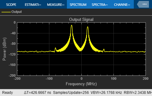
Intermodulation Analysis of Mathematical Amplifier

Uses a baseband-equivalent multitone signal as input to the Amplifier block. A Simulink® Slider Gain block enables you to vary the gain from 1 to 10.

• Open Script

Parameters

Method — Method used to model nonlinearity

Linear (default) | Cubic polynomial | Hyperbolic tangent | Saleh model | Ghorbani model | Rapp model

Method used to model the amplifier nonlinearity, specified as one of the following:

• Linear

• Cubic polynomial

• Hyperbolic tangent

• Saleh model

• Ghorbani model

• Rapp model

Tunable: Yes

Linear gain (dB) — Linear gain for output function

0 (default) | real scalar

Linear gain for the output function of the Amplifier block, specified as a real scalar in decibels.

Tunable: Yes

Dependencies

To enable this parameter, set Method to Linear, Cubic polynomial, Hyperbolic tangent, or Rapp model.

IIP3 (dBm) — Third-order input power intercept point

30 (default) | real positive number

Third-order input power intercept point for the cubic polynomial and the hyperbolic tangent amplifier model, specified as a real positive number in dBm.

Tunable: Yes

Dependencies

To enable this parameter, set Method to Cubic polynomial or Hyperbolic tangent.

AM/PM conversion (degrees per dB) — AM/PM conversion

10 (default) | scalar

AM/PM conversion for the cubic polynomial and the hyperbolic tangent amplifier model, specified as a scalar in degrees per decibel.

Tunable: Yes

Dependencies

To enable this parameter, set Method to Cubic polynomial or Hyperbolic tangent.

Lower input power limit for AM/PM conversion (dBm) — Minimum input power for which AM/PM conversion scales linearly with input power value

10 (default) | scalar

Minimum input power for which AM/PM conversion scales linearly with the input power value, specified as a scalar. Below this value, the phase shift resulting from AM/PM conversion is zero.

Tunable: Yes

Dependencies

To enable this parameter, set Method to Cubic polynomial or Hyperbolic tangent.

Upper input power limit for AM/PM conversion (dBm) — Maximum input power for which AM/PM conversion scales linearly with input power value

inf (default) | positive scalar

Maximum input power for which AM/PM conversion scales linearly with the input power value, specified as a positive scalar. Above this value, the phase shift resulting from AM/PM conversion is constant. The value of this maximum shift is given by:

$$(\text{AM/PM conversion})\cdot (\text{upper input power limit}-\text{lower input power limit}),$$

Dependencies

To enable this parameter, set Method to Cubic polynomial or Hyperbolic tangent.

Tunable: Yes

Input scaling (dB) — Number that scales input signal level

0 (default) | scalar

Number that scales the input signal level for the Saleh and Ghorbani amplifier model, specified as scalar in decibels.

Tunable: Yes

Dependencies

To enable this parameter, set Method to Saleh model or Ghorbani model.

Output scaling (dB) — Number that scales output signal level

0 (default) | scalar

Number that scales the output signal level for the Saleh and Ghorbani amplifier model, specified as scalar in decibels.

Tunable: Yes

Dependencies

To enable this parameter, set Method to Saleh model or Ghorbani model.

AM/AM parameters [alpha beta] — AM/AM parameters for Saleh amplifier model

[2.1587 1.1517] (default) | vector

AM/AM parameters for the Saleh amplifier model, specified as a vector.

Tunable: Yes

Dependencies

To enable this parameter, set Method to Saleh model.

AM/PM parameters [alpha beta] — AM/AM parameters for Saleh amplifier model

[4.0033 9.1040] (default) | vector

AM/PM parameters for the Saleh amplifier model, specified as a vector.

Tunable: Yes

Dependencies

To enable this parameter, set Method to Saleh model.

AM/AM parameters [x1 x2 x3 x4] — AM/AM parameters for Ghorbani

[8.1081 1.5413 6.5202 -0.0718] (default) | vector

AM/AM parameters for the Ghorbani amplifier model, specified as a vector.

Tunable: Yes

Dependencies

To enable this parameter, set Method to Ghorbani model.

AM/PM parameters [y1 y2 y3 y4] — AM/PM parameters for Ghorbani

[4.6645 2.0965 10.88 -0.003] (default) | vector

AM/PM parameters for the Ghorbani amplifier model, specified as a vector.

Tunable: Yes

Dependencies

To enable this parameter, set Method to Ghorbani model.

Smoothness factor — Magnitude smoothness factor

0.5 (default) | positive scalar

Magnitude smoothness factor for the Rapp amplifier model, specified as a positive scalar.

Tunable: Yes

Dependencies

To enable this parameter, set Method to Rapp model.

Output saturation level — Output saturation level

1 (default) | real positive number

Output saturation level for the Rapp amplifier model , specified as a real positive number. Scalar specifying the output saturation level.

Tunable: Yes

Dependencies

To enable this parameter, set Method to Rapp model.

Specification method — Type of noise

Noise factor (default) | Noise temperature | Noise figure

Type of noise, specified as Noise temperature, Noise figure, and Noise factor.

Tunable: Yes

Noise temperature (K) — Noise temperature to model the amplifier noise

290 (default) | nonnegative real number

Noise temperature to model the amplifier noise, specified as a nonnegative real number in kelvin.

Tunable: Yes

Dependencies

To enable this parameter, set Specification method to Noise temperature.

Noise figure (dB) — Noise figure to model amplifier noise

3.01 (default) | nonnegative real number

Noise figure to model the amplifier noise, specified as a nonnegative real number in decibels. Setting Noise figure to 0 decibels indicates a noiseless system.

Tunable: Yes

Dependencies

To enable this parameter, set Specification method to Noise figure.

Noise factor — Noise factor to model amplifier noise

2 (default) | positive integer scalar greater than or equal to 1

Noise factor to model amplifier noise relative to a noise temperature, specified as a positive integer scalar greater than or equal to 1.

To enable this parameter, set Specification method to Noise factor.

Tunable: Yes

Initial seed — Seed for random number generator

67987 (default) | nonnegative integer less than 2³²

Seed for the random number generator, specified as a nonnegative integer less than 2³². Use this value to initialize the random number generator the block uses to generate noise.

Algorithms

Modeling Nonlinearity

Use the Method parameter in the block dialog box to specify the method for modeling amplifier nonlinearity. The options for the Method parameter are

• Linear

• Cubic polynomial

• Hyperbolic tangent

• Saleh model

• Ghorbani model

• Rapp model

The linear method is implemented by a Gain block. The other nonlinear methods are implemented by subsystems underneath the block's mask. Each subsystem has the same basic structure, as shown in the following figure.

Model Parameters and Characteristics of Nonlinearity Modeling Methods

The following sections discuss how the parameters specific to the following nonlinear amplifier models affect the AM/AM and AM/PM characteristics of the Amplifier block:

• Cubic Polynomial Model

• Hyperbolic Tangent Model

• Saleh Model

• Ghorbani Model

• Rapp Model

Note

The Amplifier block also enables you to model a linear amplifier.

Cubic Polynomial Model

When you select Cubic polynomial for the nonlinearity modeling Method parameter, the Amplifier block models the AM/AM nonlinearity by:

1. Using the third-order input intercept point IIP3 (dBm) parameter to compute the factor, f, that scales the input signal before the Amplifier block applies the nonlinearity:

   $$f=\sqrt{\frac{3}{IIP3(Watts)}}=\sqrt{\frac{3}{{10}^{\left(IIP3(dBm)-30\right)/10}}}$$

2. Computing the scaled input signal by multiplying the amplifier input signal by f.

3. Limiting the scaled input signal to a maximum value of 1.

4. Applying an AM/AM conversion to the amplifier gain, according to the following cubic polynomial equation:

   $$F_{AM/AM}(u)=u-\frac{u^3}{3}$$

   where u is the magnitude of the scaled input signal, which is a unit less normalized input voltage.

The Amplifier block uses the AM/PM conversion (degrees per dB) parameter, which specifies the linear phase change, to add the AM/PM nonlinearity within the power limits specified by the Lower input power limit for AM/PM conversion (dBm) parameter and the Upper input power limit for AM/PM conversion (dBm) parameter. Outside those limits, the phase change is constant at the values corresponding to the lower and upper input power limits, which are zero and

$$(\text{AM/PM conversion})\cdot (\text{upper input power limit}-\text{lower input power limit}),$$

respectively.

The Linear gain (dB) parameter scales the output signal.

Hyperbolic Tangent Model

When you select Hyperbolic tangent for the nonlinearity modeling Method parameter, the Amplifier block computes and adds the AM/AM nonlinearity by:

1. Using the third-order input intercept point IIP3 (dBm) parameter to compute the factor, f, that scales the input signal before the Amplifier block applies the nonlinearity:

   $$f=\sqrt{\frac{3}{IIP3(Watts)}}=\sqrt{\frac{3}{{10}^{\left(IIP3(dBm)-30\right)/10}}}$$

2. Computing the scaled input signal by multiplying the amplifier input signal by f.

3. Limiting the scaled input signal to a maximum value of 1.

4. Applying an AM/AM conversion to the amplifier gain, according to the following cubic polynomial equation:

   $$F_{AM/AM}(u)=\tanh u$$

   where u is the magnitude of the scaled input signal, which is a unit less normalized input voltage.

The Amplifier block uses the AM/PM conversion (degrees per dB) parameter, which specifies the linear phase change, to add the AM/PM nonlinearity within the power limits specified by the Lower input power limit for AM/PM conversion (dBm) parameter and the Upper input power limit for AM/PM conversion (dBm) parameter. Outside those limits, the phase change is constant at the values corresponding to the lower and upper input power limits, which are zero and

$$(\text{AM/PM conversion})\cdot (\text{upper input power limit}-\text{lower input power limit}),$$

respectively.

The Linear gain (dB) parameter scales the output signal.

Saleh Model

When you select Saleh model for the nonlinearity modeling Method parameter, the Input scaling (dB) parameter scales the input signal before the nonlinearity is applied. The block multiplies the input signal by the parameter value, converted from decibels to linear units. If you set the parameter to be the inverse of the input signal amplitude, the scaled signal has amplitude normalized to 1.

The AM/AM parameters, alpha and beta, are used to compute the amplitude gain for an input signal using the following function

$$F_{AM/AM}(u)=\frac{\alpha u}{1+\beta u^2}$$

where u is the magnitude of the scaled signal.

The AM/PM parameters, alpha and beta, are used to compute the phase change for an input signal using the following function

$$F_{AM/PM}(u)=\frac{\alpha u^2}{1+\beta u^2}$$

where u is the magnitude of the input signal. Note that the AM/AM and AM/PM parameters, although similarly named alpha and beta, are distinct.

The Output scaling (dB) parameter scales the output signal similarly.

Ghorbani Model

When you select Ghorbani model for the nonlinearity modeling Method parameter, the Input scaling (dB) parameter scales the input signal before the nonlinearity is applied. The block multiplies the input signal by the parameter value, converted from decibels to linear units. If you set the parameter to be the inverse of the input signal amplitude, the scaled signal has amplitude normalized to 1.

The AM/AM parameters, [x₁ x₂ x₃ x₄], are used to compute the amplitude gain for an input signal using the following function

$$F_{AM/AM}(u)=\frac{x_1{u}^{x_2}}{1+x_3{u}^{x_2}}+x_{4}u$$

where u is the magnitude of the scaled signal.

The AM/PM parameters, [y₁ y₂ y₃ y₄], are used to compute the phase change for an input signal using the following function

$$F_{AM/PM}(u)=\frac{y_1{u}^{y_2}}{1+y_3{u}^{y_2}}+y_{4}u$$

where u is the magnitude of the scaled signal.

The Output scaling (dB)parameter scales the output signal similarly.

Rapp Model

When you select Rapp model for the nonlinearity modeling Method parameter, the Smoothness factor and Output saturation level parameters are used to compute the amplitude gain for an input signal by the following function

$$F_{AM/AM}(u)=\frac{u}{{\left(1+{\left(\frac{u}{O_{sat}}\right)}^{2S}\right)}^{\frac{1}{2S}}}$$

where u is the magnitude of the scaled signal, S is the Smoothness factor and O_sat is the Output saturation level.

The Rapp model does not apply a phase change to the input signal.

The Output saturation level parameter limits the output signal level. The Smoothness factor parameter controls the transition for the amplitude gain as the input amplitude approaches saturation. The smaller the smoothness factor, the smoother the curve.

AM/AM and AM/PM Conversions

The subsystems for the nonlinear methods implement the AM/AM and AM/PM conversions differently, according to the nonlinearity method you specify. To see exactly how the Amplifier block implements the conversions for a specific method, you can view the AM/AM and AM/PM subsystems that implement these conversions as follows:

1. Right-click the Amplifier block.

2. Select Look under mask in the pop-up menu. This displays the block's configuration underneath the mask. The block contains five subsystems corresponding to the five nonlinearity methods.

3. Double-click the subsystem for the method in which you are interested. A subsystem displays similar to the one shown in the preceding figure.

4. Double-click one of the subsystems labeled AM/AM or AM/PM to view how the block implements the conversions.

The following figure shows, for the Saleh method, plots of

• Output voltage against input voltage for the AM/AM conversion

• Output phase against input voltage for the AM/PM conversion

  

Thermal Noise Simulation

You can specify the amount of thermal noise in three ways, according to the Specification method parameter you select.

• Noise temperature — Specifies the noise in kelvin.

• Noise factor — Specifies the noise by the following equation:

  $$\text{Noise factor = }1+\frac{\text{Noise temperature}}{290}$$

• Noise figure — Specifies the noise in decibels relative to a noise temperature of 290 kelvin. In terms of noise factor,

  Noise figure = 10log(Noise factor)

  (1)

  Note

  Some RF blocks require the sample time to perform baseband modeling calculations. To ensure the accuracy of these calculations, the Input Port block, as well as the mathematical RF blocks, compare the input sample time to the sample time you provide in the mask. If they do not match, or if the input sample time is missing because the blocks are not connected, an error message appears.

Application of Nonlinearity

All five subsystems for the nonlinear Method options apply a memoryless nonlinearity to the complex baseband input signal. Each one

1. Multiplies the signal by a gain factor.

2. Splits the complex signal into its magnitude and angle components.

3. Applies an AM/AM conversion to the magnitude of the signal, according to the selected nonlinearity method, to produce the magnitude of the output signal.

4. Applies an AM/PM conversion to the phase of the signal, according to the selected nonlinearity method, and adds the result to the angle of the signal to produce the angle of the output signal.

5. Combines the new magnitude and angle components into a complex signal and multiplies the result by a gain factor, which is controlled by the Linear gain (dB) parameter.

References

[1] Ghorbani, A. and M. Sheikhan, “The Effect of Solid State Power Amplifiers (SSPAs) Nonlinearities on MPSK and M-QAM Signal Transmission,” Sixth Int'l Conference on Digital Processing of Signals in Comm., 1991, pp. 193-197.

[2] Rapp, C., “Effects of HPA-Nonlinearity on a 4-DPSK/OFDM-Signal for a Digital Sound Broadcasting System,” in Proceedings of the Second European Conference on Satellite Communications, Liege, Belgium, Oct. 22-24, 1991, pp. 179-184.

[3] Saleh, A.A.M., “Frequency-independent and frequency-dependent nonlinear models of TWT amplifiers,” IEEE Trans. Communications, vol. COM-29, pp.1715-1720, November 1981.

Version History

Introduced before R2006a