Create a Simple Model

You can use Simulink^® to model a system and then simulate the dynamic behavior of that system. In this example, you create a simple model, but you can use the same basic techniques to create complex models. The example simulates the simplified motion of a car. A car is typically in motion while the gas pedal is pressed. After the pedal is released, the car slows to a stop and idles.

A Simulink block is a model element that defines a mathematical relationship between its input and output. To create this simple model, you need four Simulink blocks.

Block Name	Block Purpose	Model Purpose
Pulse Generator	Generate an input signal for the model.	Represent the accelerator pedal.
Gain	Multiply the input signal by a constant value.	Calculate how pressing the accelerator affects the car acceleration.
Second-Order Integrator	Integrate the input signal twice.	Obtain the position from acceleration.
Outport	Designate a signal as an output from the model.	Designate the position as an output from the model.

Simulating this model integrates a brief pulse twice to get a ramp. The input pulse represents a press of the gas pedal: 1 when the pedal is pressed and 0 when it is not. The output ramp is the increasing distance from the starting point.

Open New Model

Use the Simulink Editor to build your models.

1. Start MATLAB^®. From the MATLAB Toolstrip, click the Simulink button .

   

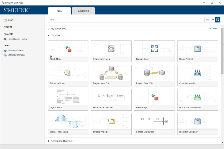
2. Select the Blank Model template.

   The Simulink Editor opens.

   To avoid shadowing, or having more than one model with the same name open at once, the Simulink Editor checks loaded models and files on the path and creates a model with the next available name: untitled, untitled1, untitled2, and so on.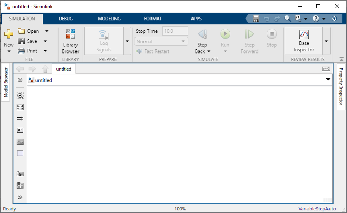

   

3. On the Simulation tab, select Save > Save as. In the File name text box, enter a name for your model, for example, simple_model. Click Save. The model is saved with the file extension .slx.

Open Simulink Library Browser

Simulink provides a set of block libraries that are organized by functionality in the Library Browser. These libraries are common to most workflows:

• Continuous — Blocks for systems with continuous states

• Discrete — Blocks for systems with discrete states

• Math Operations — Blocks that implement algebraic and logical equations

• Sinks — Blocks that store and show the signals that connect to them

• Sources — Blocks that generate the signal values that drive the model

To open the Library Browser, in the Simulink Toolstrip, on the Simulation tab, click Library Browser.

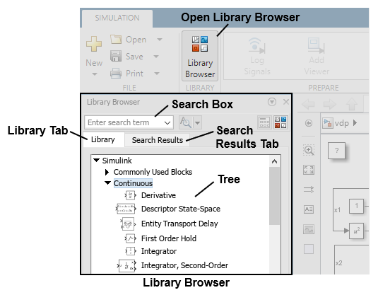
To browse through the block libraries, in the library tree, expand a library and its sublibraries.

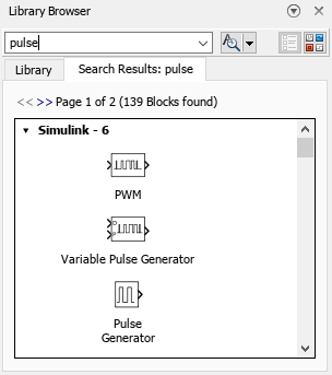
To search all of the available block libraries, enter a search term. For example, find the Pulse Generator block. In the search box, enter pulse, then press Enter. The software searches the libraries for blocks with pulse in their name or description and then displays the blocks on the Search Results tab of the Library Browser. You can return to browsing the library tree by clicking the Library tab.

Add Blocks to Model

To start building the model, add blocks to the model canvas. You can add blocks using the Library Browser or the quick insert menu.

1. Add a Pulse Generator block. In the Library Browser tree, expand the Simulink library. Expand the Sources sublibrary. Drag the Pulse Generator block to the model canvas.

   

2. Add a Gain block. Double-click the model canvas. In the quick insert menu that appears, enter gain. A list of blocks appears.

   

   Multiple different blocks can have the same name, provided they are stored in different library files. The libraries to which a block belongs are listed under the block name. Check that the Gain block from the Simulink library is selected. If not, select the block using your arrow keys or by clicking the block name.

   To learn about the selected block, read the description in the details pane to the right of the search results. To see the full documentation for the block, click Documentation. For examples involving the block, click the links under Examples. To hide or unhide the details pane, click the arrow in the upper right.

   Add the selected block to the model by pressing Enter or double-clicking the selection.

   

3. Add these blocks to the model using the Library Browser or the quick insert menu.

   Block	Library
   Out1	Simulink library, Sinks sublibrary
   Second-Order Integrator	Simulink library, Continuous sublibrary

4. Add a second Out1 block by copying the existing one and pasting it at another point using the keyboard shortcuts Ctrl+C and Ctrl+V (on macOS, use command+C and command+V). Your model now has the blocks you need.

Connect Blocks

Connect the:

• Pulse Generator block to the Gain block.

• Gain block to Second-Order Integrator block.

• Second-Order Integrator block to the two Out1 blocks.

For example, to connect the Pulse Generator block to the Gain block:

1. Click the output port on the right side of the Pulse Generator block.

   The output port and all input ports suitable for a connection are indicated by a blue chevron symbol (>).

2. To see the connection cue, point to the chevron symbol (>).

3. Click the cue to connect the blocks with a line and an arrow that indicates the direction of signal flow.

For more information about how to connect blocks, see Connect Blocks.

Once you have connected the blocks, line up the Pulse Generator, Gain, and Second-Order Integrator blocks by dragging each block. To resize a block, drag a corner of the block.

For large models, instead of dragging the individual blocks, you can improve the model layout using auto-arrange. Right-click the model canvas. The Top Model context menu appears. In Simulink context menus, formatting options such as changing colors or fonts, or auto-arranging the model, are located in the format bar. To expand the format bar, at the top of the menu, click the arrow . Then, click the Auto Arrange button .

Tip

To view a tooltip that explains what action you can take by pushing a context menu button, pause your pointer on the button icon.

Auto-arrange aligns the blocks and straightens the signal lines.

Edit Block Parameter Values

Blocks have parameter values that you can modify. To find out which parameters you can modify for a block and what type of values the parameters take, open the block documentation. Right-click the block, and in the upper right corner of the context menu, click the Open help documentation button .

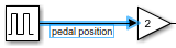
For some blocks, such as Constant blocks or Gain blocks, you can change a parameter value directly on the face of the block. Change the gain value of the Gain block in the example model to 2. Select the block, click the value on the block, enter the new value, and then press Enter.

You can also change the gain value in the Block Parameters dialog box. To open the Block Parameters dialog box, double-click the block. Alternatively, right-click the block, and then click the Block Parameters button . In the dialog box that opens, change the Gain value to 2 and press Enter.

A third option is to use the Property Inspector. Select the Gain block. To open the Property Inspector, press Ctrl+Shift+I (on macOS, press command+option+O). Alternatively, right-click the block, and then click the Property Inspector button . In the Property Inspector, on the Parameters tab, change the Gain value to 2.

To change parameter values not displayed on the block icon, use the Block Parameters dialog box or the Property Inspector. If you do not see the name of a parameter whose value you want to change in the Block Parameters dialog box, check the Property Inspector, and vice versa.

Run Simulation

Specify the stop time for the simulation. Then, simulate the model.

1. On the Simulation tab, set the simulation stop time. In the Simulink Toolstrip, on the Simulation tab, enter the value in the Stop Time text box.

   

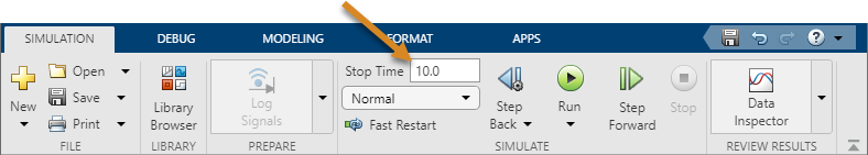
   The default stop time of 10.0 is appropriate for this model. This time value has no units. The time unit in a Simulink simulation depends on how the equations are constructed. This example simulates the simplified motion of a car for 10 seconds, but other models could have time units in milliseconds or years.

2. To simulate the model, press Ctrl+T (on macOS, press command+T). Alternatively, in the toolstrip, on the Simulation tab, click Run .

View Simulation Data

To view simulation results in the Simulation Data Inspector, right-click one of the signal lines, and then click the View in Data Inspector button .

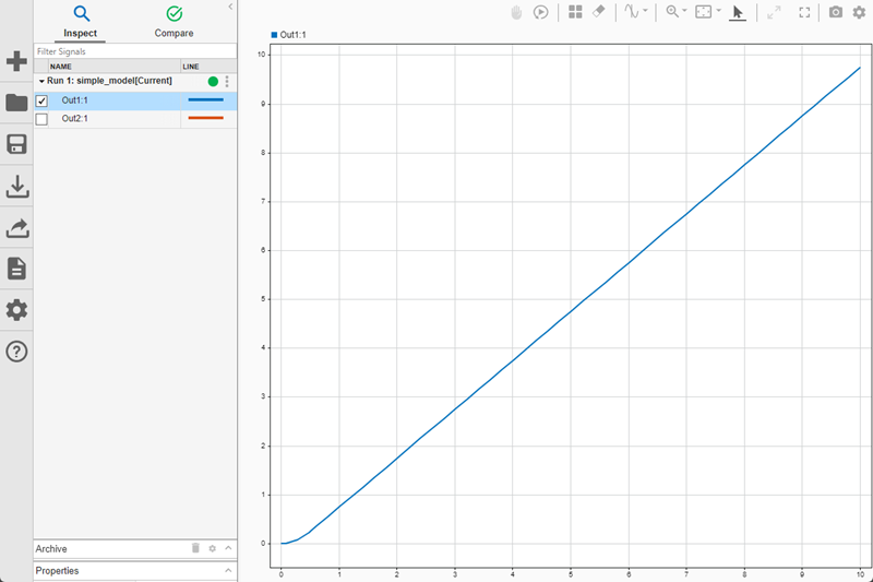
To plot data in the Simulation Data Inspector, select signals from the checklist on the left. For example, to plot the position of the car, select the signal named Out1:1.

Refine Model

You can refine a model by changing the block parameters, adding new blocks, making new connections, and annotating signal lines.

Change Block Parameters

This example models a proximity sensor based on an existing motion model named moving_car.

In this scenario, a digital sensor measures the distance between the car and an obstacle 10 m (30 ft) away. The model outputs the sensor measurement and the position of the car, taking these conditions into consideration:

• The car comes to a hard stop when it reaches the obstacle.

• In the physical world, a sensor measures the distance imprecisely, causing random numerical errors.

• A digital sensor operates at fixed time intervals.

Open the moving_car model.

open_system("moving_car.slx");

You first need to model the hard stop when the car position reaches 10. The Integrator, Second-Order block has a parameter for that purpose.

1. Double-click the Integrator, Second-Order block. The Block Parameters dialog box appears.

2. Select Limit x and enter 10 for Upper limit x. The background color for the parameter changes to indicate a modification that is not applied to the model. Click OK to apply the changes and close the dialog box.

Add New Blocks and Connections

Modify the model to add a sensor that measures the distance from the obstacle. Expand the model window to accommodate the new blocks as necessary.

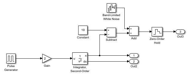
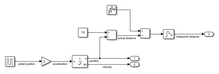
• To find the distance between the vehicle and obstacle position, add a Constant block from the Sources library and set the value of block to 10. To find the distance between the obstacle position and the vehicle position, add the Subtract block from the Math Operations library.

• To simulate the imperfect measurements of a real sensor, add noise to the model by using the Band-Limited White Noise block from the Sources library. Double-click the block to set the Noise power parameter to 0.001. Add the noise to the distance measurement by using an Add block from the Math Operations library.

• In Simulink, sampling of a signal at a given interval requires a sample and hold. Add the Zero-Order Hold block from the Discrete library. Then, double-click the block to change the Sample Time parameter to 0.1.

• To log the sensor output, connect the Zero-Order Hold block to another Outport block.

Connect the new blocks. The output of the Second-Order Integrator block is already connected to another port. To create a branch in that signal, left-click the signal to highlight potential ports for connection, and click the appropriate port.

Annotate Signals

Add signal names to the model.

1. Double-click the signal and type the signal name.

   

2. To finish, click away from the text box.

3. Repeat these steps to add the names as shown.

   

View Multiple Signals

Compare the actual distance signal with the measured distance signal. The measured distance signal is logged as output. To log the actual distance signal, you can mark it for signal logging. Right-click the signal line, and then click the Log Signals button . A logging badge indicates that the signal is marked for logging.

Simulate the model. To view simulation results in the Simulation Data Inspector, right-click the signal line, and then click the View in Data Inspector button . Expand the Outports and Signals checklists. To plot both signals on the same time plot, select the actual distance and measured distance signals.

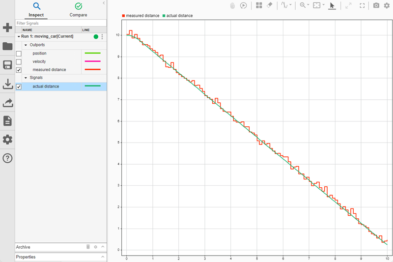
The plot shows that the measurement can deviate from the actual value by as much as 0.3 m. This information is useful when designing safety features, such as a collision warning.

View Signals on Separate Subplots

You can also analyze results by viewing signals on separate subplots. For example, you can add subplots for the pedal position and velocity signals to view the relationship between the pedal position, the velocity of the car, and the distance between the car and the obstacle.

Mark the pedal position signal for signal logging. Right-click the pedal position signal line, and then click the Log Signals button .

Simulate the model. When the simulation finishes, in the Simulation Data Inspector, click Visualizations and layouts . Then, create a 3-by-1 layout by specifying the number of rows and columns in the grid.

Add the velocity signal to the middle subplot and the pedal position signal to the bottom subplot. To add a signal to a subplot, select the subplot, and then select the signal from the signal table.

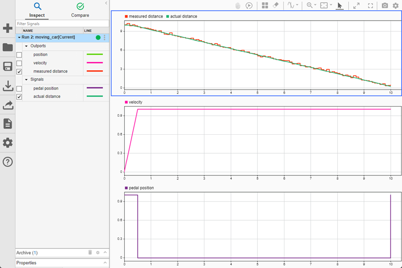
Visualizing the data on three subplots lets you to see the how pressing the gas pedal affects the velocity of the car and its distance from the obstacle. To explore this further, you can change the behavior of the gas pedal by adjusting the parameters of the Pulse Generator block. To open the Block Parameters dialog box for the Pulse Generator block, double-click the block. For example, model pressing the gas pedal for one second twice by setting Period to 5 and Pulse Width to 20.

Simulate the model. In the Simulation Data Inspector, press the space bar to fit the signals to view.

In the Simulation Data Inspector, you can further inspect the data by customizing the plot and signal appearance, zooming and panning, and adding data cursors. For more information, see Create Plots Using the Simulation Data Inspector.