anova1
One-way analysis of variance
Syntax
Description
p = anova1(y)y and returns the p-value.
anova1 treats each column of y as a
separate group. The function tests the hypothesis that the samples in the columns of
y are drawn from populations with the same mean against the
alternative hypothesis that the population means are not all the same. The function
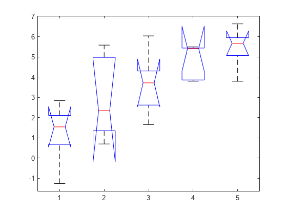
also displays the box plot for each group
in y and the standard ANOVA table
(tbl).
p = anova1(y,group,displayopt)displayopt is 'on' (default)
and suppresses the displays when displayopt is 'off'.
[ returns a structure, p,tbl,stats]
= anova1(___)stats,
which you can use to perform a multiple comparison test. A multiple
comparison test enables you to determine which pairs of group means
are significantly different. To perform this test, use multcompare, providing the stats structure
as an input argument.
Examples
Create sample data matrix y with columns that are constants, plus random normal disturbances with mean 0 and standard deviation 1.
y = meshgrid(1:5);
rng default; % For reproducibility
y = y + normrnd(0,1,5,5)
y = 5×5

    1.5377    0.6923    1.6501    3.7950    5.6715
    2.8339    1.5664    6.0349    3.8759    3.7925
   -1.2588    2.3426    3.7254    5.4897    5.7172
    1.8622    5.5784    2.9369    5.4090    6.6302
    1.3188    4.7694    3.7147    5.4172    5.4889
Perform one-way ANOVA.
p = anova1(y)
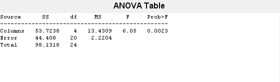
p =
0.0023
The ANOVA table shows the between-groups variation (Columns) and within-groups variation (Error). SS is the sum of squares, and df is the degrees of freedom. The total degrees of freedom is total number of observations minus one, which is 25 - 1 = 24. The between-groups degrees of freedom is number of groups minus one, which is 5 - 1 = 4. The within-groups degrees of freedom is total degrees of freedom minus the between groups degrees of freedom, which is 24 - 4 = 20.
MS is the mean squared error, which is SS/df for each source of variation. The F-statistic is the ratio of the mean squared errors (13.4309/2.2204). The p-value is the probability that the test statistic can take a value greater than the value of the computed test statistic, i.e., P(F > 6.05). The small p-value of 0.0023 indicates that differences between column means are significant.
Input the sample data.
strength = [82 86 79 83 84 85 86 87 74 82 ...
            78 75 76 77 79 79 77 78 82 79];
alloy = {'st','st','st','st','st','st','st','st',...
         'al1','al1','al1','al1','al1','al1',...
         'al2','al2','al2','al2','al2','al2'};
The data are from a study of the strength of structural beams in Hogg (1987). The vector strength measures deflections of beams in thousandths of an inch under 3000 pounds of force. The vector alloy identifies each beam as steel ('st'), alloy 1 ('al1'), or alloy 2 ('al2'). Although alloy is sorted in this example, grouping variables do not need to be sorted.
Test the null hypothesis that the steel beams are equal in strength to the beams made of the two more expensive alloys. Turn the figure display off and return the ANOVA results in a cell array.
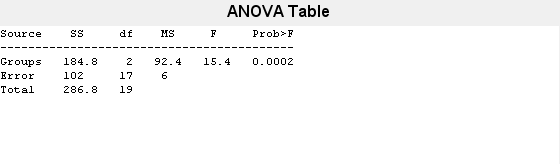
[p,tbl] = anova1(strength,alloy,'off')p = 1.5264e-04
tbl=4×6 cell array
    {'Source'}    {'SS'      }    {'df'}    {'MS'      }    {'F'       }    {'Prob>F'    }
    {'Groups'}    {[184.8000]}    {[ 2]}    {[ 92.4000]}    {[ 15.4000]}    {[1.5264e-04]}
    {'Error' }    {[102.0000]}    {[17]}    {[  6.0000]}    {0×0 double}    {0×0 double  }
    {'Total' }    {[286.8000]}    {[19]}    {0×0 double}    {0×0 double}    {0×0 double  }
The total degrees of freedom is total number of observations minus one, which is . The between-groups degrees of freedom is number of groups minus one, which is . The within-groups degrees of freedom is total degrees of freedom minus the between groups degrees of freedom, which is .
MS is the mean squared error, which is SS/df for each source of variation. The F-statistic is the ratio of the mean squared errors. The p-value is the probability that the test statistic can take a value greater than or equal to the value of the test statistic. The p-value of 1.5264e-04 suggests rejection of the null hypothesis.
You can retrieve the values in the ANOVA table by indexing into the cell array. Save the F-statistic value and the p-value in the new variables Fstat and pvalue.
Fstat = tbl{2,5}Fstat = 15.4000
pvalue = tbl{2,6}pvalue = 1.5264e-04
Input the sample data.
strength = [82 86 79 83 84 85 86 87 74 82 ...
            78 75 76 77 79 79 77 78 82 79];
alloy = {'st','st','st','st','st','st','st','st',...
         'al1','al1','al1','al1','al1','al1',...
         'al2','al2','al2','al2','al2','al2'};
The data are from a study of the strength of structural beams in Hogg (1987). The vector strength measures deflections of beams in thousandths of an inch under 3000 pounds of force. The vector alloy identifies each beam as steel (st), alloy 1 (al1), or alloy 2 (al2). Although alloy is sorted in this example, grouping variables do not need to be sorted.
Perform one-way ANOVA using anova1. Return the structure stats, which contains the statistics multcompare needs for performing Multiple Comparisons.
[~,~,stats] = anova1(strength,alloy);
The small p-value of 0.0002 suggests that the strength of the beams is not the same.
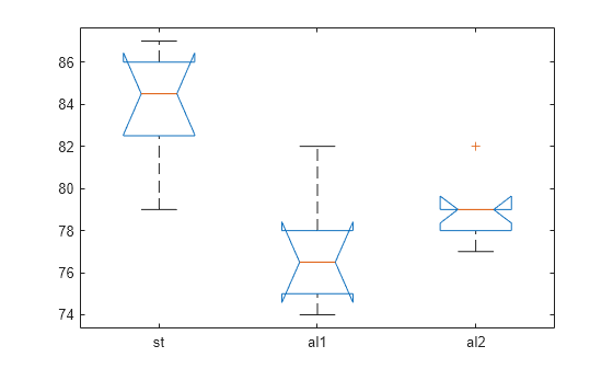
Perform a multiple comparison of the mean strength of the beams.
[c,~,~,gnames] = multcompare(stats);
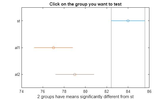
In the figure, the blue bar represents the comparison interval for mean material strength for steel. The red bars represent the comparison intervals for the mean material strength for alloy 1 and alloy 2. Neither of the red bars overlaps with the blue bar, which indicates that the mean material strength for steel is significantly different from that of alloy 1 and alloy 2. You can confirm the significant difference by clicking the bars that represent alloy 1 and 2.
Display the multiple comparison results and the corresponding group names in a table.
tbl = array2table(c,"VariableNames", ...
    ["Group A","Group B","Lower Limit","A-B","Upper Limit","P-value"]);
tbl.("Group A") = gnames(tbl.("Group A"));
tbl.("Group B") = gnames(tbl.("Group B"))
tbl=3×6 table
    Group A    Group B    Lower Limit    A-B    Upper Limit     P-value
    _______    _______    ___________    ___    ___________    __________

    {'st' }    {'al1'}      3.6064        7       10.394       0.00016831
    {'st' }    {'al2'}      1.6064        5       8.3936        0.0040464
    {'al1'}    {'al2'}      -5.628       -2        1.628          0.35601
The first two columns show the pair of groups that are compared. The fourth column shows the difference between the estimated group means. The third and fifth columns show the lower and upper limits for the 95% confidence intervals of the true difference of means. The sixth column shows the p-value for a hypothesis that the true difference of means for the corresponding groups is equal to zero.
The first two rows show that both comparisons involving the first group (steel) have confidence intervals that do not include zero. Because the corresponding p-values (1.6831e-04 and 0.0040, respectively) are small, those differences are significant.
The third row shows that the differences in strength between the two alloys is not significant. A 95% confidence interval for the difference is [-5.6,1.6], so you cannot reject the hypothesis that the true difference is zero. The corresponding p-value of 0.3560 in the sixth column confirms this result.
Input Arguments
Sample data, specified as a vector or matrix.
If
yis a vector, you must specify thegroupinput argument. Each element ingrouprepresents a group name of the corresponding element iny. Theanova1function treats theyvalues corresponding to the same value ofgroupas part of the same group. Use this design when groups have different numbers of elements (unbalanced ANOVA).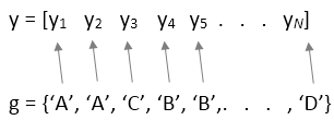
If
yis a matrix and you do not specifygroup, thenanova1treats each column ofyas a separate group. In this design, the function evaluates whether the population means of the columns are equal. Use this design when each group has the same number of elements (balanced ANOVA).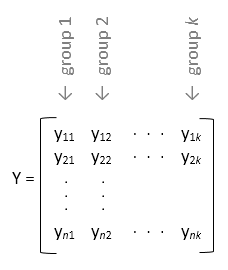
If
yis a matrix and you specifygroup, then each element ingrouprepresents a group name for the corresponding column iny. Theanova1function treats the columns that have the same group name as part of the same group.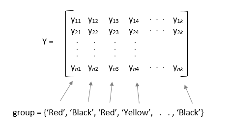
Note
anova1 ignores any NaN values
in y. Also, if group contains
empty or NaN values, anova1
ignores the corresponding observations in y. The
anova1 function performs balanced ANOVA if each
group has the same number of observations after the function disregards
empty or NaN values. Otherwise,
anova1 performs unbalanced ANOVA.
Data Types: single | double
Grouping variable containing group names, specified as a numeric vector, logical vector, categorical vector, character array, string array, or cell array of character vectors.
If
yis a vector, then each element ingrouprepresents a group name of the corresponding element iny. Theanova1function treats theyvalues corresponding to the same value ofgroupas part of the same group.N is the total number of observations.
If
yis a matrix, then each element ingrouprepresents a group name for the corresponding column iny. Theanova1function treats the columns ofythat have the same group name as part of the same group.If you do not want to specify group names for the matrix sample data
y, enter an empty array ([]) or omit this argument. In this case,anova1treats each column ofyas a separate group.
If group contains empty or NaN
values, anova1 ignores the corresponding observations
in y.
For more information on grouping variables, see Grouping Variables.
Example: 'group',[1,2,1,3,1,...,3,1] when y is a vector
with observations categorized into groups 1, 2, and 3
Example: 'group',{'white','red','white','black','red'} when
y is a matrix with five columns categorized into
groups red, white, and black
Data Types: single | double | logical | categorical | char | string | cell
Indicator to display the ANOVA table and box plot, specified as 'on' or
'off'. When displayopt is
'off', anova1 returns the output
arguments, only. It does not display the standard ANOVA table and box
plot.
Example: p = anova(x,group,'off')
Output Arguments
More About
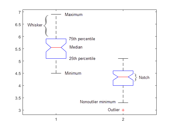
anova1 returns a box plot of the observations for each
group in y. Box plots provide a visual comparison of the group
location parameters.
On each box, the central mark is the median (2nd quantile,
q2) and the edges of the box are the
25th and 75th percentiles (1st and 3rd quantiles,
q1 and
q3, respectively). The whiskers extend
to the most extreme data points that are not considered outliers. The outliers are
plotted individually using the '+' symbol. The extremes of the
whiskers correspond to q3 + 1.5 ×
(q3 –
q1) and q1 – 1.5 ×
(q3 –
q1).
Box plots include notches for the comparison of the median values. Two medians are
significantly different at the 5% significance level if their intervals, represented
by notches, do not overlap. This test is different from the
F-test that ANOVA performs; however, large differences in the
center lines of the boxes correspond to a large F-statistic value
and correspondingly a small p-value. The extremes of the notches
correspond to q2 –
1.57(q3 –
q1)/sqrt(n) and
q2 +
1.57(q3 –
q1)/sqrt(n), where
n is the number of observations without any
NaN values. In some cases, notches can extend outside the
boxes.
For more information about box plots, see 'Whisker' and 'Notch' of boxplot.
Alternative Functionality
Instead of using anova1, you can create an anova
object by using the anova function.
The anova function provides these advantages:
The
anovafunction allows you to specify the ANOVA model type, sum of squares type, and factors to treat as categorical.anovaalso supports table predictor and response input arguments.In addition to the outputs returned by
anova1, the properties of theanovaobject contain the following:ANOVA model formula
Fitted ANOVA model coefficients
Residuals
Factors and response data
The
anovaobject functions allow you to conduct further analysis after fitting theanovaobject. For example, you can create an interactive plot of multiple comparisons of means for the ANOVA, get the mean response estimates for each value of a factor, and calculate the variance component estimates.
References
[1] Hogg, R. V., and J. Ledolter. Engineering Statistics. New York: MacMillan, 1987.
Version History
Introduced before R2006a
See Also
anova | anova2 | anovan | boxplot | multcompare