CensoredLinearModel

Censored linear regression model

Since R2025a

Description

A CensoredLinearModel object contains the results of fitting a linear regression model to censored data. An observation is censored if at least one bound on its value is known while the exact value remains unknown.

Use the properties of a CensoredLinearModel object to investigate a fitted censored linear regression model. The object properties include information about coefficient estimates, summary statistics, residuals, and censoring. Use the object functions to predict responses, generate random values, and visualize the linear regression model.

Creation

Create a CensoredLinearModel object using fitlmcens.

Properties

Coefficient Estimates

CoefficientCovariance — Covariance matrix of coefficient estimates

Read-only: numeric matrix

This property is read-only.

Covariance matrix of coefficient estimates, represented as a p-by-p matrix of numeric values. p is the number of coefficients in the fitted model, as given by NumCoefficients.

For details, see Coefficient Standard Errors and Confidence Intervals.

Data Types: single | double

CoefficientNames — Coefficient names

Read-only: cell array of character vectors

This property is read-only.

Coefficient names, represented as a cell array of character vectors, each containing the name of the corresponding term.

Data Types: cell

Coefficients — Coefficient values

Read-only: table

This property is read-only.

Coefficient values, represented as a table that contains one row for each coefficient and these columns:

• Estimate — Estimated coefficient value

• SE — Standard error of the estimate

• tStat — t-statistic for a two-sided test with the null hypothesis that the coefficient is zero

• pValue — p-value for the t-statistic

Use coefCI to find the confidence intervals of the coefficient estimates.

To obtain any of these columns as a vector, index into the property using dot notation. For example, obtain the estimated coefficient vector in the model mdl:

beta = mdl.Coefficients.Estimate

Data Types: table

NumCoefficients — Number of model coefficients

Read-only: positive integer

This property is read-only.

Number of model coefficients, represented as a positive integer. NumCoefficients includes coefficients that are set to zero when the model terms are rank deficient.

Data Types: double

Summary Statistics

DFE — Degrees of freedom for error

Read-only: positive integer

This property is read-only.

Degrees of freedom for the error (residuals), equal to the number of observations minus the number of estimated coefficients, represented as a positive integer.

Data Types: double

Fitted — Fitted response values based on input data

Read-only: numeric vector

This property is read-only.

Fitted (predicted) response values based on the input data, represented as an n-by-1 numeric vector. n is the number of observations in the input data. Use predict to calculate predictions for other predictor values, or to compute confidence bounds on Fitted.

Data Types: single | double

LogLikelihood — Loglikelihood of response values

Read-only: numeric scalar

This property is read-only.

Loglikelihood of the response values, represented as a numeric scalar. The loglikelihood is based on the assumption that each response value follows a normal distribution. The mean of the normal distribution is the fitted (predicted) response value, and the estimated variance is mdl.Sigma².

Data Types: single | double

ModelCriterion — Criterion for model comparison

Read-only: structure

This property is read-only.

Criterion for model comparison, represented as a structure with these fields:

• AIC — Akaike information criterion. AIC = –2*logL + 2*m, where logL is the loglikelihood and m is the number of estimated parameters.

• AICc — Akaike information criterion corrected for the sample size. AICc = AIC + (2*m*(m + 1))/(n – m – 1), where n is the number of observations.

• BIC — Bayesian information criterion. BIC = –2*logL + m*log(n).

• CAIC — Consistent Akaike information criterion. CAIC = –2*logL + m*(log(n) + 1).

Information criteria are model selection tools that you can use to compare multiple models fit to the same data. These criteria are likelihood-based measures of model fit that include a penalty for complexity (specifically, the number of parameters). Different information criteria are distinguished by the form of the penalty.

When you compare multiple models, the model with the lowest information criterion value is the best-fitting model. The best-fitting model can vary depending on the criterion used for model comparison.

To obtain any of the criterion values as a scalar, index into the property using dot notation. For example, obtain the AIC value aic in the model mdl:

aic = mdl.ModelCriterion.AIC

Data Types: struct

ModelFitVsConstantModel — Chi-square statistic of regression model

Read-only: structure

This property is read-only.

Chi-square statistic of the linear regression model vs. the constant model, represented as a structure. The constant model is a linear regression model that includes an intercept only.

The ModelFitVsConstantModel structure contains these fields:

• Chi2Stat — Chi-square statistic of the fitted model versus the constant model.

• Pval — p-value for the chi-square statistic.

• LogLConstant — Loglikelihood for the constant model. This statistic is used to calculate the loglikelihood vs. constant model statistic in the model display.

Data Types: struct

Rsquared — Pseudo R-squared values for fitted model

Read-only: structure

This property is read-only.

Pseudo R-squared values for the fitted model, represented as a structure. Each field of Rsquared contains a pseudo R-squared value calculated with a different formula [1].

Field	Description
'McFadden'	The McFadden value is $$R^2=1-\frac{\ln (L_{Full})}{\ln (L_{Null})},$$ where $$L_{Full}$$ is the loglikelihood of the fitted model, and $$L_{Null}$$ is the loglikelihood of a model with no predictors.
'AdjustedMcFadden'	The adjusted McFadden value is $$R^2=1-\frac{\ln (L_{Full})-K}{\ln (L_{Null})},$$ where K is the number of model coefficients in $$L_{Full}$$.

Data Types: struct

Residuals — Residuals for fitted model

Read-only: table

This property is read-only.

Residuals for the fitted model, represented as a table that contains one row for each observation and the following columns:

• Raw — Observed minus fitted values

• Standardized — Standardized residuals given by the formula $$\widehat{\sigma }\sqrt{N/N-p}$$, where $$\widehat{\sigma }\sqrt{N/N-p}$$ is the estimated standard deviation in mdl.Sigma, N is the number of observations, and p is the number of predictors in the model

Use plotResiduals to create a plot of the residuals. For details, see Residuals.

Rows with missing values (in ObservationInfo.Missing) or excluded values (in ObservationInfo.Excluded) are not used in the fit. These rows contain NaN values.

To obtain either column as a vector, index into the property using dot notation. For example, obtain the raw residual vector r in the model mdl:

r = mdl.Residuals.Raw

Data Types: table

Sigma — Estimate for error standard deviation

Read-only: numeric scalar

This property is read-only.

Estimate for the error standard deviation, represented as a numeric scalar.

Data Types: single | double

Input Data

Formula — Model information

LinearFormula object

This property is read-only after object creation.

Model information, represented as a LinearFormula object.

Display the formula of the fitted model mdl using dot notation:

mdl.Formula

NumObservations — Number of observations

positive integer

This property is read-only after object creation.

Number of observations used to fit the model, represented as a positive integer. NumObservations is the number of observations supplied in the original table or matrix, minus any excluded rows or rows with missing values. To exclude rows, set with the ExcludeObservations name-value argument when you create the object with fitlmcens.

Data Types: double

NumPredictors — Number of predictor variables

positive integer

This property is read-only after object creation.

Number of predictor variables used to fit the model, represented as a positive integer.

Data Types: double

NumRightCensored — Number of right-censored observations

positive integer

This property is read-only after object creation.

Number of right-censored observations, represented as a positive integer.

Data Types: double

NumLeftCensored — Number of left-censored observations

positive integer

This property is read-only after object creation.

Number of left-censored observations, represented as a positive integer.

Data Types: double

NumIntervalCensored — Number of interval-censored observations

positive integer

This property is read-only after object creation.

Number of interval-censored observations, represented as a positive integer.

Data Types: double

NumUncensored — Number of uncensored observations

positive integer

This property is read-only after object creation.

Number of uncensored observations, represented as a positive integer.

Data Types: double

NumVariables — Number of variables

positive integer

This property is read-only after object creation.

Number of variables in the input data, represented as a positive integer. NumVariables is the number of variables in the original table, or the total number of columns in the predictor matrix and response vector.

NumVariables also includes any variables not used to fit the model as predictors or as the response.

Data Types: double

ObservationInfo — Observation information

table

This property is read-only after object creation.

Observation information, represented as an n-by-4 or n-by-5 table, where n is the number of rows of input data. ObservationInfo contains the columns described below.

Column	Description
Weights	Observation weights, specified as a numeric value. The default value is 1.
Excluded	Indicator of excluded observations, specified as a logical value. The value is true if you exclude the observation from the fit by setting the ExcludeObservations name-value argument when you create the model object using fitlmcens.
Missing	Indicator of missing observations, specified as a logical value. The value is true if the observation is missing.
Subset	Indicator of whether fitlmcens uses the observation, specified as a logical value. The value is true if the observation is not excluded or missing, meaning the function uses the observation.
Censoring	Indicator of how the observation is censored. The entry -1 indicates left-censoring, the entry 1 indicates right-censoring, and the entry 0 indicates no censoring. ObservationInfo contains this column only if you specify Censoring=cens when you create the model using fitlmcens.

To obtain any of these columns as a vector, index into the property using dot notation. For example, obtain the weights vector w of the model mdl:

w = mdl.ObservationInfo.Weights

Data Types: table

ObservationNames — Observation names

cell array of character vectors

This property is read-only after object creation.

Observation names, returned as a cell array of character vectors containing the names of the observations used to fit the model.

• If the fit is based on a table containing observation names, this property contains those names.

• Otherwise, this property is an empty cell array.

Data Types: cell

PredictorNames — Names of predictors used to fit model

cell array of character vectors

This property is read-only after object creation.

Names of predictors used to fit the model, represented as a cell array of character vectors.

Data Types: cell

ResponseName — Response variable name

character vector

This property is read-only after object creation.

Response variable name, represented as a character vector.

Data Types: char

VariableInfo — Information about variables

table

This property is read-only after object creation.

Information about the variables contained in Variables, represented as a table with one row for each variable and the columns described below.

Column	Description
Class	Variable class, specified as a cell array of character vectors, such as 'double' and 'categorical'
Range	Variable range, specified as a cell array of vectors Continuous variable — Two-element vector [min,max], the minimum and maximum values Categorical variable — Vector of distinct variable values
InModel	Indicator of which variables are in the fitted model, specified as a logical vector. The value is true if the model includes the variable.
IsCategorical	Indicator of categorical variables, specified as a logical vector. The value is true if the variable is categorical.

VariableInfo also includes any variables not used to fit the model as predictors or as the response.

Data Types: table

VariableNames — Names of variables

cell array of character vectors

This property is read-only after object creation.

Names of the variables, returned as a cell array of character vectors.

• If the fit is based on a table, this property contains the names of the variables in the table.

• If the fit is based on a predictor matrix and response vector, this property contains the values specified by the VarNames name-value argument of the fitting method. The default value of VarNames is {'x1','x2',...,'xn','y'}.

VariableNames also includes any variables not used to fit the model as predictors or as the response.

Data Types: cell

Variables — Input data

table

This property is read-only after object creation.

Input data, returned as a table. Variables contains both predictor and response values.

• If the fit is based on a table, this property contains all the data from the table.

• Otherwise, this property is a table created from the input data matrix X and the response vector y.

Variables also includes any variables not used to fit the model as predictors or as the response.

Data Types: table

Object Functions

compact	Create compact censored linear regression model
plotResiduals	Plot residuals of censored linear regression model
plotSlice	Plot of slices through fitted censored linear regression surface
predict	Predict responses of censored linear regression model
partialDependence	Compute partial dependence
plotPartialDependence	Create partial dependence plot (PDP) and individual conditional expectation (ICE) plots
feval	Predict responses of censored linear regression model using one input for each predictor
random	Simulate responses with random noise for censored linear regression model
coefCI	Confidence intervals of coefficient estimates for censored linear regression model
coefTest	Linear hypothesis test on censored linear regression model coefficients

Examples

Fit Linear Regression Model to Censored Table Data

Load the readmissiontimes sample data.

load readmissiontimes

The variables Age, Weight, and ReadmissionTime contain data for patient age, weight, and time of readmission. The Censored variable contains censoring information for ReadmissionTime.

Save Age, Weight, and ReadmissionTime in a table.

tbl = table(Age,Weight,ReadmissionTime);

Fit a censored linear regression model using Age, Weight, and Smoker as the predictor variables, ReadmissionTime as the response, and Censored as the censoring information. Because ReadmissionTime is the last column in tbl, you do not need to specify the ResponseVarName argument.

mdl1 = fitlmcens(tbl,Censoring=Censored)

mdl1 = 
Censored linear regression model
    ReadmissionTime ~ 1 + Age + Weight

Estimated Coefficients:
                   Estimate        SE        tStat        pValue  
                   _________    ________    ________    __________

    (Intercept)        28.62      3.5313      8.1047    1.7047e-12
    Age            -0.060686    0.061984    -0.97905       0.33001
    Weight          -0.11977    0.017199     -6.9638    4.1162e-10

Sigma: 4.245

Number of observations: 100, Error degrees of freedom: 96
25 right-censored observations
75 uncensored observations
Likelihood ratio statistic vs. constant model: 39, p-value = 3.47e-09

mdl1 is a CensoredLinearModel object that includes the results of fitting a censored linear regression model to the data. The output display includes information about the model, statistics for each model term, and the censored observations. The p-values for the Weight and Age terms indicate that Weight has a statistically significant effect on patient readmission time and Age does not.

Fit another model to the data, using only the Weight term.

mdl2 = fitlmcens(tbl,"ReadmissionTime~Weight",Censoring=Censored)

mdl2 = 
Censored linear regression model
    ReadmissionTime ~ 1 + Weight

Estimated Coefficients:
                   Estimate      SE        tStat       pValue  
                   ________    _______    _______    __________

    (Intercept)      26.398     2.7107     9.7387    4.9168e-16
    Weight         -0.12041    0.01729    -6.9642    3.9554e-10

Sigma: 4.273

Number of observations: 100, Error degrees of freedom: 97
25 right-censored observations
75 uncensored observations
Likelihood ratio statistic vs. constant model: 38, p-value = 7.06e-10

The result for Likelihood ratio statistic vs. constant model shows that mdl2 is a slightly better fit than mdl1.

Analyze Residuals

Load the censoreddata sample data.

load censoreddata.mat

The matrix X contains data for three predictors, and the matrix yint contains bounds for a censored response variable.

Fit a linear regression model to the censored data in X and yint.

mdl = fitlmcens(X,yint);

Display a probability plot of the standardized residuals.

plotResiduals(mdl,"probability",ResidualType="standardized")

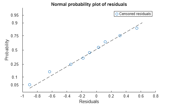
The plot shows that the standardized residuals have a normal distribution (approximately).

Plot Regression Surface

Load the readmissiontimes sample data.

load readmissiontimes

The variables Age, Weight, Smoker, and ReadmissionTime contain data for patient age, weight, smoking status, and time of readmission. The Censored variable contains censoring information for ReadmissionTime.

Save Age, Weight, Smoker, ReadmissionTime, and Censored in a table.

tbl = table(Age,Weight,Smoker,ReadmissionTime,Censored);

Fit a censored linear regression model using Age, Weight, and Smoker as the predictor variables, ReadmissionTime as the response, and Censored as the censoring information. Specify that smoker is a categorical variable.

mdl = fitlmcens(tbl,"ReadmissionTime",Censoring="Censored",CategoricalVars="Smoker");

Display the estimates, standard errors, t-statistics, and p-values for the model coefficients.

mdl.Coefficients

ans=4×4 table
                   Estimate        SE        tStat        pValue  
                   _________    ________    ________    __________

    (Intercept)        27.74      3.4008      8.1569    1.4048e-12
    Age            -0.053476    0.059514    -0.89854       0.37117
    Weight          -0.11101    0.016823     -6.5986    2.3484e-09
    Smoker_1         -2.3455     0.93105     -2.5192      0.013434

The p-values for the coefficients indicate that not enough evidence exists to conclude that age has a statistically significant effect on patient readmission time. Note that the model does not contain a coefficient corresponding to Smoker=0, indicating that nonsmokers are the reference category.

Generate new predictor data from the ranges for Age and Weight using the meshgrid function.

[ageNew,weightNew] = meshgrid(25:50,100:200);

Save the coefficient estimates for the fitted model in a variable named coefs, and display the model formula.

coefs = mdl.Coefficients.Estimate;
mdl.Formula

ans = 
ReadmissionTime ~ 1 + Age + Weight + Smoker

Create a vector of indices for the observations in the fitting data that correspond to smokers. Generate new response data for smokers using the model formula and coefs.

idx = Smoker==1;
resNew = coefs(1) + coefs(2)*ageNew + coefs(3)*weightNew + coefs(4);

Use the surf and scatter3 functions to plot a surface of the new data together with the fitting data, and the fitted responses corresponding to smokers.

surf(ageNew,weightNew,resNew,FaceAlpha=0.2,FaceColor="k",EdgeColor="none") %    Regression surface

hold on

scatter3(Age(idx),Weight(idx),ReadmissionTime(idx),"x",SizeData=30) %   Data used to fit the model
scatter3(Age(idx),Weight(idx),mdl.Fitted(idx),"Filled",SizeData=30) %   Fitted response data

legend("Regression surface","Fitted values","Data")
xlabel("Age")
ylabel("Weight")
zlabel("Readmission Time")
view(-85,20)

The plot shows the fitted responses in blue on the gray response surface. The surface passes through the bulk of the data used to fit the model, shown with red x markers.

References

[1] Allison, P. D. Measures of Fit for Logistic Regression. Statistical Horizons LLC and the University of Pennsylvania, 2014.

[2] Law, M., and Jackson, D. Residual Plots for Linear Regression Models with Censored Outcome Data: A Refined Method for Visualizing Residual Uncertainty, Communications in Statistics - Simulation and Computation, vol. 46, no. 4, pp. 3159–71, 2017.

Version History

Introduced in R2025a