loss

R2026b

Loss of neural network incremental learning model on batch of data

Since R2026b

Syntax

L = loss(Mdl,X,Y)

L = loss(Mdl,X,Y,Name=Value)

Description

loss returns the regression or classification loss of a configured incremental learning model for neural network regression (incrementalRegressionNeuralNetwork object) or classification (incrementalClassificationNeuralNetwork object).

To measure model performance on a data stream and store the results in the output model, call updateMetrics or updateMetricsAndFit.

L = loss(Mdl,X,Y) returns the loss for the incremental learning model Mdl using the batch of predictor data X and corresponding responses Y.

L = loss(Mdl,X,Y,Name=Value) uses additional options specified by one or more name-value arguments. For example, you can specify observation weights and a custom loss function.

Examples

Measure Model Performance During Incremental Learning

The performance of an incremental model on streaming data is measured in three ways:

• Cumulative metrics measure the performance since the start of incremental learning.

• Window metrics measure the performance on a specified window of observations. The metrics are updated every time the model processes the specified window.

• The loss function measures the performance on a specified batch of data only.

Load the human activity data set. Randomly shuffle the data.

load humanactivity
n = numel(actid);
rng(0,"twister") % For reproducibility
idx = randsample(n,n);
X = feat(idx,:);
Y = actid(idx);

For details on the data set, enter Description at the command line.

Create a neural network classification model for incremental learning. Specify the class names, a metrics window size of 1000 observations, and track the classification error metric. Configure the model for loss by fitting it to the first 10 observations.

Mdl = incrementalClassificationNeuralNetwork(ClassNames=unique(Y), ...
    MetricsWindowSize=1000,Metrics="classiferror");
initobs = 10;
Mdl = fit(Mdl,X(1:initobs,:),Y(1:initobs));

Mdl is an incrementalClassificationNeuralNetwork model.

Simulate a data stream, and perform the following actions on each incoming chunk of 100 observations:

1. Call updateMetrics to measure the cumulative performance and the performance within a window of observations. Overwrite the previous incremental model with a new one to track performance metrics.

2. Call loss to measure the model performance on the incoming chunk.

3. Call fit to fit the model to the incoming chunk. Overwrite the previous incremental model with a new one fitted to the incoming observations.

4. Store all performance metrics to see how they evolve during incremental learning.

% Preallocation
numObsPerChunk = 100;
nchunk = floor((n - initobs)/numObsPerChunk);
mc = array2table(zeros(nchunk,3),VariableNames=["Cumulative","Window","Chunk"]);

% Incremental learning
for j = 1:nchunk
    ibegin = min(n,numObsPerChunk*(j-1) + 1 + initobs);
    iend   = min(n,numObsPerChunk*j + initobs);
    idx = ibegin:iend;    
    Mdl = updateMetrics(Mdl,X(idx,:),Y(idx));
    mc{j,["Cumulative","Window"]} = Mdl.Metrics{"ClassificationError",:};
    mc{j,"Chunk"} = loss(Mdl,X(idx,:),Y(idx));
    Mdl = fit(Mdl,X(idx,:),Y(idx));
end

Mdl is an incrementalClassificationNeural model object trained on all the data in the stream. During incremental learning and after the model is warmed up, updateMetrics checks the performance of the model on the incoming observations, and then the fit function fits the model to those observations. loss is agnostic of the metrics warm-up period, so it measures the classification error for every chunk.

To see how the performance metrics evolve during training, plot them.

plot(mc.Variables)
xlim([0 nchunk])
ylabel("Classification Error")
xline((Mdl.TrainingOptions.TuningPeriod+Mdl.MetricsWarmupPeriod) ...
    /numObsPerChunk,"--")
grid on
legend(mc.Properties.VariableNames)
xlabel("Iteration")

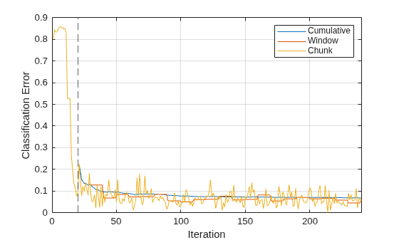
The yellow line represents the classification error on each incoming chunk of data. After the solver tuning period and the metrics warm-up period (vertical dashed line), Mdl tracks the cumulative and window metrics.

Compute Loss Using Observation Weights

The performance of an incremental model on streaming data is measured in three ways:

• Cumulative metrics measure the performance since the start of incremental learning.

• Window metrics measure the performance on a specified window of observations. The metrics are updated every time the model processes the specified window.

• The loss function measures the performance on a specified batch of data only.

Load and Preprocess Data

Load the human activity data set. Randomly shuffle the data.

load humanactivity
rng(0,"twister"); % For reproducibility
n = numel(actid);
idx = randsample(n,n);
X = feat(idx,:);
Y = actid(idx);

For details on the data set, enter Description at the command line.

Suppose that the data from a stationary subject (Y <= 2) has double the quality of the data from a moving subject. Create a weight variable that assigns a weight of 2 to observations from a stationary subject and 1 to a moving subject.

W = ones(n,1) + (Y <=2);

Train Neural Network Classification Model

Fit a neural network classification model to a random sample of half the data. Specify observation weights.

idxtt = randsample([true false],n,true);
TTMdl = fitcnet(X(idxtt,:),Y(idxtt),Weights=W(idxtt))

TTMdl = 
  ClassificationNeuralNetwork
             ResponseName: 'Y'
    CategoricalPredictors: []
               ClassNames: [1 2 3 4 5]
           ScoreTransform: 'none'
          NumObservations: 12039
               LayerSizes: 10
              Activations: 'relu'
    OutputLayerActivation: 'softmax'
                   Solver: 'LBFGS'
          ConvergenceInfo: [1×1 struct]
          TrainingHistory: [1000×7 table]


  Properties, Methods

TTMdl is a ClassificationNeuralNetwork model object representing a traditionally trained neural network classification model.

Convert Trained Model

Convert the traditionally trained model to a model for incremental learning. Specify to use the FreeRex solver, a metrics warm-up period of 1000 observations, and to track the classification error metric.

IncrementalMdl = incrementalLearner(TTMdl, ...
    TrainingOptions=incrementalTrainingOptions("freerex"), ...
    MetricsWarmupPeriod=1000,Metrics="classiferror")

IncrementalMdl = 
  incrementalClassificationNeuralNetwork

                   IsWarm: 0
                  Metrics: [2×2 table]
               ClassNames: [1 2 3 4 5]
           ScoreTransform: 'none'
               LayerSizes: 10
              Activations: "relu"
    OutputLayerActivation: "softmax"
                   Solver: "freerex"


  Properties, Methods

IncrementalMdl is an incrementalClassificationNeuralNetwork model. Because class names are specified in IncrementalMdl.ClassNames, labels encountered during incremental learning must be in IncrementalMdl.ClassNames.

Separately Track Performance Metrics and Fit Model

Perform incremental learning on the rest of the data by using the updateMetrics and fit functions. For incremental learning, orient the observations of the predictor data in columns. At each iteration:

1. Simulate a data stream by processing 50 observations at a time.

2. Call updateMetrics to update the cumulative and window classification error of the model given the incoming chunk of observations. Overwrite the previous incremental model to update the losses in the Metrics property. Note that the function does not fit the model to the chunk of data—the chunk is "new" data for the model. Specify that the observations are oriented in columns, and specify the observation weights.

3. Store the classification error.

4. Call loss to measure the model performance on the incoming chunk. Specify that the observations are oriented in columns, and specify the observation weights.

5. Call fit to fit the model to the incoming chunk of observations. Overwrite the previous incremental model to update the model parameters. Specify that the observations are oriented in columns, and specify the observation weights.

% Preallocation
idxil = ~idxtt;
nil = sum(idxil);
numObsPerChunk = 50;
nchunk = floor(nil/numObsPerChunk);
mc = array2table(zeros(nchunk,3),VariableNames=["Cumulative","Window","Chunk"]);

Xil = X(idxil,:)';
Yil = Y(idxil);
Wil = W(idxil);

% Incremental learning
for j = 1:nchunk
    ibegin = min(nil,numObsPerChunk*(j-1) + 1);
    iend   = min(nil,numObsPerChunk*j);
    idx = ibegin:iend; 
    IncrementalMdl = updateMetrics(IncrementalMdl,Xil(:,idx),Yil(idx), ...
        Weights=Wil(idx),ObservationsIn="columns");
    mc{j,["Cumulative","Window"]} = IncrementalMdl.Metrics{"ClassificationError",:};
    mc{j,"Chunk"} = loss(IncrementalMdl,Xil(:,idx),Yil(idx), ...
        Weights=Wil(idx),ObservationsIn="columns");
    IncrementalMdl = fit(IncrementalMdl,Xil(:,idx),Yil(idx), ...
        Weights=Wil(idx),ObservationsIn="columns");
end

IncrementalMdl is an incrementalClassificationNeuralNetwork model object trained on all the data in the stream.

Alternatively, you can use updateMetricsAndFit to update performance metrics of the model given a new chunk of data, and then fit the model to the data.

Plot a trace plot of the performance metrics.

plot(mc.Variables)
xlim([0 nchunk])
xline(IncrementalMdl.MetricsWarmupPeriod/numObsPerChunk,"r-.");
legend(mc.Properties.VariableNames)
ylabel("Classification Error")
xlabel("Iteration")

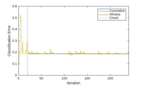
The yellow line represents the classification error on each incoming chunk of data. After the metrics warm-up period (vertical dashed line), Mdl tracks the cumulative and window metrics.

Input Arguments

Mdl — Incremental learning model

incrementalClassificationNeuralNetwork model object | incrementalRegressionNeuralNetwork model object

Incremental learning model, specified as an incrementalClassificationNeuralNetwork or incrementalRegressionNeuralNetwork model object. You can create Mdl directly or by converting a supported, traditionally trained machine learning model using the incrementalLearner function. For more details, see the corresponding reference page.

To generate predictions, the model must be trained. That is, you must pass Mdl and data to fit or updateMetricsAndFit before calling loss, or convert a traditionally trained model using incrementalLearner.

X — Chunk of predictor data

floating-point matrix

Chunk of predictor data, specified as a floating-point matrix of n observations and Mdl.NumPredictors predictor variables. The value of the ObservationsIn name-value argument determines the orientation of the variables and observations. The default ObservationsIn value is "rows", which indicates that observations in the predictor data are oriented along the rows of X.

The length of the observation labels Y and the number of observations in X must be equal; Y(j) is the label of observation j (row or column) in X.

Note

• loss supports only floating-point input predictor data. If your input data includes categorical data, you must prepare an encoded version of the categorical data. Use dummyvar to convert each categorical variable to a numeric matrix of dummy variables. Then, concatenate all dummy variable matrices and any other numeric predictors. For more details, see Dummy Variables.

Data Types: single | double

Y — Chunk of responses (labels)

categorical array | character array | string array | logical vector | floating-point vector | cell array of character vectors

Chunk of responses (labels), specified as a categorical, character, or string array, a logical or floating-point vector, or a cell array of character vectors for classification problems; or a floating-point vector for regression problems.

The length of the observation responses Y and the number of observations in X must be equal; Y(j) is the response of observation j (row or column) in X.

For classification problems, loss issues an error when one or both of these conditions are met:

• Y contains a new label and the maximum number of classes has already been reached (see the ClassNames and MaxNumClasses arguments of incrementalClassificationNeuralNetwork).

• The ClassNames property of the input model Mdl is nonempty, and the data types of Y and Mdl.ClassNames are different.

Data Types: char | string | cell | categorical | logical | single | double

Name-Value Arguments

Specify optional pairs of arguments as Name1=Value1,...,NameN=ValueN, where Name is the argument name and Value is the corresponding value. Name-value arguments must appear after other arguments, but the order of the pairs does not matter.

Example: LossFun=@customLoss,Weights=W specifies a custom loss function and observation weights.

LossFun — Loss function

string vector | function handle | cell vector | structure array

Loss function, specified as a built-in loss function name or function handle.

• Classification problems: The following table lists the available loss functions when Mdl is an incrementalClassificationNeuralNetwork model. Specify one using its corresponding character vector or string scalar.

  Name	Description
  "binodeviance"	Binomial deviance
  "classiferror"	Classification error
  "crossentropy"	Cross-entropy loss
  "exponential"	Exponential loss
  "hinge"	Hinge loss
  "logit"	Logistic loss
  "mincost" (default)	Minimum expected misclassification cost
  "quadratic"	Quadratic loss

  For more details, see Classification Loss

  To specify a custom loss function, use function handle notation. The function must have this form:

  lossval = lossfcn(C,S,W,Cost)

  • The output argument lossval is an n-by-1 floating-point vector, where n is the number of observations in X. The value in lossval(j) is the classification loss of observation j.

  • You specify the function name (lossfcn).

  • C is an n-by-K logical matrix with rows indicating the class to which the corresponding observation belongs. K is the number of distinct classes (numel(Mdl.ClassNames), and the column order corresponds to the class order in the ClassNames property. Create C by setting C(p,q) = 1, if observation p is in class q, for each observation in the specified data. Set the other element in row p to 0.

  • S is an n-by-K numeric matrix of predicted classification scores. S is similar to the Posterior output of predict, where rows correspond to observations in the data and the column order corresponds to the class order in the ClassNames property. S(p,q) is the classification score of observation p being classified in class q.

  • W is an n-by-1 numeric vector of observation weights.

  • Cost is a K-by-K numeric matrix of misclassification costs.

• Regression problems: You must specify LossFun as "mse" (weighted mean squared error) or a custom loss function when Mdl is an incrementalRegressionNeuralNetwork model. The function must have this form:

  lossval = lossfun(Y,YFit,W)

  • The output argument lossval is a floating-point scalar.

  • You specify the function name (lossfun).

  • If Mdl is a model with one response variable, then Y is a length-n numeric vector of observed responses, where n is the number of observations in Tbl or X. If Mdl is a model with multiple response variables, then Y is an n-by-k numeric matrix of observed responses, where k is the number of response variables.

  • YFit is a length-n numeric vector or an n-by-k numeric matrix of corresponding predicted responses. The size of YFit must match the size of Y.

  • W is an n-by-1 numeric vector of observation weights.

Example: LossFun="mse"

Example: LossFun=@lossfcn

Data Types: char | string | function_handle

ObservationsIn — Predictor data observation dimension

"rows" (default) | "columns"

Predictor data observation dimension, specified as "rows" or "columns".

Example: ObservationsIn="columns"

Data Types: char | string

OutputType — Type of output loss

"average" (default) | "per-response"

Type of output loss, specified as "average" or "per-response". You can only specify OutputType when Mdl is an incrementalRegressionNeuralNetwork model object.

Value	Description
"average"	loss averages the loss values across all response variables and returns a scalar value.
"per-response"	loss returns a vector, where each element is the loss for one response variable.

Example: OutputType="per-response"

Data Types: char | string

StandardizeResponses — Flag to standardize response data

false or 0 (default) | true or 1

Flag to standardize the response data before computing the loss, specified as a numeric or logical 0 (false) or 1 (true). If you set StandardizeResponses to true, then the software centers and scales each response variable by the corresponding variable mean and standard deviation in the training data. You can only specify StandardizeReponses when Mdl is an incrementalRegressionNeuralNetwork model object.

Specify StandardizeResponses as true when you have multiple response variables with very different scales and OutputType is "average".

Example: StandardizeResponses=true

Data Types: single | double | logical

Weights — Chunk of observation weights

floating-point vector of positive values

Chunk of observation weights, specified as a floating-point vector of positive values. loss weighs the observations in X with the corresponding values in Weights. The size of Weights must equal n, which is the number of observations in X.

By default, Weights is ones(n,1).

For more details, including normalization schemes, see Observation Weights.

Example: Weights=W specifies the observation weights as the vector W.

Data Types: double | single

Output Arguments

L — Classification or regression loss

numeric scalar

Classification or regression loss, returned as a numeric scalar. The interpretation of L depends on Weights and LossFun.

More About

Classification Loss

Classification loss functions measure the predictive inaccuracy of classification models. When you compare the same type of loss among many models, a lower loss indicates a better predictive model.

Consider the following scenario.

• L is the weighted average classification loss.

• n is the sample size.

• For binary classification:

  • y_j is the observed class label. The software codes it as –1 or 1, indicating the negative or positive class (or the first or second class in the ClassNames property), respectively.

  • f(X_j) is the positive-class classification score for observation (row) j of the predictor data X.

  • m_j = y_jf(X_j) is the classification score for classifying observation j into the class corresponding to y_j. Positive values of m_j indicate correct classification and do not contribute much to the average loss. Negative values of m_j indicate incorrect classification and contribute significantly to the average loss.

• For algorithms that support multiclass classification (that is, K ≥ 3):

  • y_j ^* is a vector of K – 1 zeros, with 1 in the position corresponding to the true, observed class y_j . For example, if the true class of the second observation is the third class and K = 4, then y ₂ ^* = [0 0 1 0]′. The order of the classes corresponds to the order in the ClassNames property of the input model.

  • f(X_j ) is the length K vector of class scores for observation j of the predictor data X. The order of the scores corresponds to the order of the classes in the ClassNames property of the input model.

  • m_j = y_j ^*′f(X_j ). Therefore, m_j is the scalar classification score that the model predicts for the true, observed class.

• The weight for observation j is w_j . The software normalizes the observation weights so that they sum to the corresponding class weights (prior probabilities) specified by the Prior name-value argument. Therefore,

  $${\displaystyle \sum _{j=1}^n{w}_j}=1.$$

Given this scenario, the following table describes the supported loss functions that you can specify by using the LossFun name-value argument.

Loss Function	Value of LossFun	Equation
Binomial deviance	"binodeviance"	$$L={\displaystyle \sum _{j=1}^n{w}_j\log \left\{1+\exp \left[-2m_j\right]\right\}}.$$
Observed misclassification cost	"classifcost"	$$L={\displaystyle \sum _{j=1}^n{w}_j}{c}_{y_j{\widehat{y}}_j},$$ where $${\widehat{y}}_j$$ is the class label corresponding to the class with the maximal score, and $$c_{y_j{\widehat{y}}_j}$$ is the user-specified cost of classifying an observation into class $${\widehat{y}}_j$$ when its true class is yj.
Misclassified rate in decimal	"classiferror"	$$L={\displaystyle \sum _{j=1}^n{w}_j}I\left\{{\widehat{y}}_j\ne y_j\right\},$$ where I{·} is the indicator function.
Cross-entropy loss	"crossentropy"	"crossentropy" is appropriate only for neural network models. The weighted cross-entropy loss is $$L=-{\displaystyle \sum _{j=1}^n\frac{{\tilde{w}}_j\log (m_j)}{Kn}},$$ where the weights $${\tilde{w}}_j$$ are normalized to sum to n instead of 1.
Exponential loss	"exponential"	$$L={\displaystyle \sum _{j=1}^n{w}_j\exp \left(-m_j\right)}.$$
Hinge loss	"hinge"	$$L={\displaystyle \sum }_{j=1}^n{w}_j\max \left\{0,1-m_j\right\}.$$
Logistic loss	"logit"	$$L={\displaystyle \sum _{j=1}^n{w}_j\log \left(1+\exp \left(-m_j\right)\right)}.$$
Minimal expected misclassification cost	"mincost"	"mincost" is appropriate only if classification scores are posterior probabilities. The software computes the weighted minimal expected classification cost using this procedure for observations j = 1,...,n. Estimate the expected misclassification cost of classifying the observation Xj into the class k: $${\gamma }_{jk}={\left(f{\left(X_j\right)}^{\prime }C\right)}_k.$$ f(Xj) is the column vector of class posterior probabilities for the observation Xj. C is the cost matrix stored in the Cost property of the model. For observation j, predict the class label corresponding to the minimal expected misclassification cost: $${\widehat{y}}_j=\underset{k=1,\mathrm{...},K}{\text{argmin}}{\gamma }_{jk}.$$ Using C, identify the cost incurred (cj) for making the prediction. The weighted average of the minimal expected misclassification cost loss is $$L={\displaystyle \sum _{j=1}^n{w}_j{c}_j}.$$
Quadratic loss	"quadratic"	$$L={\displaystyle \sum _{j=1}^n{w}_j{\left(1-m_j\right)}^2}.$$

If you use the default cost matrix (whose element value is 0 for correct classification and 1 for incorrect classification), then the loss values for "classifcost", "classiferror", and "mincost" are identical. For a model with a nondefault cost matrix, the "classifcost" loss is equivalent to the "mincost" loss most of the time. These losses can be different if prediction into the class with maximal posterior probability is different from prediction into the class with minimal expected cost. Note that "mincost" is appropriate only if classification scores are posterior probabilities.

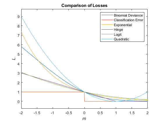
This figure compares the loss functions (except "classifcost", "crossentropy", and "mincost") over the score m for one observation. Some functions are normalized to pass through the point (0,1).

Algorithms

Observation Weights

For classification problems, if the prior class probability distribution is known (in other words, the prior distribution is not empirical), loss normalizes observation weights to sum to the prior class probabilities in the respective classes. This action implies that observation weights are the respective prior class probabilities by default.

For regression problems or if the prior class probability distribution is empirical, the software normalizes the specified observation weights to sum to 1 each time you call loss.

Version History

Introduced in R2026b