fitted

Fitted responses from a linear mixed-effects model

Syntax

yfit = fitted(lme)

yfit = fitted(lme,Name,Value)

Description

yfit = fitted(lme) returns the fitted conditional response from the linear mixed-effects model lme.

yfit = fitted(lme,Name,Value) returns the fitted response from the linear mixed-effects model lme with additional options specified by one or more Name,Value pair arguments.

For example, you can specify if you want to compute the fitted marginal response.

Examples

Compute Fitted Conditional and Marginal Responses

Load the sample data.

load flu

The flu dataset array has a Date variable, and 10 variables containing estimated influenza rates (in 9 different regions, estimated from Google® searches, plus a nationwide estimate from the Center for Disease Control and Prevention, CDC).

To fit a linear-mixed effects model, your data must be in a properly formatted dataset array. To fit a linear mixed-effects model with the influenza rates as the responses and region as the predictor variable, combine the nine columns corresponding to the regions into an array. The new dataset array, flu2, must have the response variable, FluRate, the nominal variable, Region, that shows which region each estimate is from, and the grouping variable Date.

flu2 = stack(flu,2:10,'NewDataVarName','FluRate','IndVarName','Region');
flu2.Date = nominal(flu2.Date);

Fit a linear mixed-effects model with fixed effects for region and a random intercept that varies by Date.

Region is a categorical variable. You can specify the contrasts for categorical variables using the DummyVarCoding name-value pair argument when fitting the model. When you do not specify the contrasts, fitlme uses the 'reference' contrast by default. Because the model has an intercept, fitlme takes the first region, NE, as the reference and creates eight dummy variables representing the other eight regions. For example, $$I[MidAtl]$$ is the dummy variable representing the region MidAtl. For details, see Dummy Variables.

The corresponding model is

$$\begin{array}{l}{y}_{im}={\beta }_0+{\beta }_{1}I{\left[MidAtl\right]}_i+{\beta }_{2}I{\left[ENCentral\right]}_i+{\beta }_{3}I{\left[WNCentral\right]}_i+{\beta }_{4}I{\left[SAtl\right]}_i\\ +{\beta }_{5}I{\left[ESCentral\right]}_i+{\beta }_{6}I{\left[WSCentral\right]}_i+{\beta }_{7}I{\left[Mtn\right]}_i+{\beta }_{8}I{\left[Pac\right]}_i+b_{0m}+{\epsilon }_{im},m=1,2,...,52,\end{array}$$

where $$y_{im}$$ is the observation $$i$$ for level $$m$$ of grouping variable Date, $${\beta }_j$$, $$j$$ = 0, 1, ..., 8, are the fixed-effects coefficients, with $${\beta }_0$$ being the coefficient for region NE. $$b_{0m}$$ is the random effect for level $$m$$ of the grouping variable Date, and $${\epsilon }_{im}$$ is the observation error for observation $$i$$. The random effect has the prior distribution, $$b_{0m}\sim N(0,{\sigma }_b^2)$$ and the error term has the distribution, $${\epsilon }_{im}\sim N(0,{\sigma }^2)$$.

lme = fitlme(flu2,'FluRate ~ 1 + Region + (1|Date)')

lme = 
Linear mixed-effects model fit by ML

Model information:
    Number of observations             468
    Fixed effects coefficients           9
    Random effects coefficients         52
    Covariance parameters                2

Formula:
    FluRate ~ 1 + Region + (1 | Date)

Model fit statistics:
    AIC       BIC       LogLikelihood    Deviance
    318.71    364.35    -148.36          296.71  

Fixed effects coefficients (95% CIs):
    Name                        Estimate    SE          tStat      DF     pValue        Lower        Upper    
    {'(Intercept)'     }          1.2233    0.096678     12.654    459     1.085e-31       1.0334       1.4133
    {'Region_MidAtl'   }        0.010192    0.052221    0.19518    459       0.84534    -0.092429      0.11281
    {'Region_ENCentral'}        0.051923    0.052221     0.9943    459        0.3206    -0.050698      0.15454
    {'Region_WNCentral'}         0.23687    0.052221     4.5359    459    7.3324e-06      0.13424      0.33949
    {'Region_SAtl'     }        0.075481    0.052221     1.4454    459       0.14902     -0.02714       0.1781
    {'Region_ESCentral'}         0.33917    0.052221      6.495    459    2.1623e-10      0.23655      0.44179
    {'Region_WSCentral'}           0.069    0.052221     1.3213    459       0.18705    -0.033621      0.17162
    {'Region_Mtn'      }        0.046673    0.052221    0.89377    459       0.37191    -0.055948      0.14929
    {'Region_Pac'      }        -0.16013    0.052221    -3.0665    459     0.0022936     -0.26276    -0.057514

Random effects covariance parameters (95% CIs):
Group: Date (52 Levels)
    Name1                  Name2                  Type           Estimate    Lower     Upper  
    {'(Intercept)'}        {'(Intercept)'}        {'std'}        0.6443      0.5297    0.78368

Group: Error
    Name               Estimate    Lower      Upper
    {'Res Std'}        0.26627     0.24878    0.285

The $$p$$-values 7.3324e-06 and 2.1623e-10 respectively show that the fixed effects of the flu rates in regions WNCentral and ESCentral are significantly different relative to the flu rates in region NE.

The confidence limits for the standard deviation of the random-effects term, $${\sigma }_b$$, do not include 0 (0.5297, 0.78368), which indicates that the random-effects term is significant. You can also test the significance of the random-effects terms using the compare method.

The conditional fitted response from the model at a given observation includes contributions from fixed and random effects. For example, the estimated best linear unbiased predictor (BLUP) of the flu rate for region WNCentral in week 10/9/2005 is

$$\begin{array}{l}{\underset{}{\overset{ˆ}{y}}}_{WNCentral,10/9/2005}={\underset{}{\overset{ˆ}{\beta }}}_0+{\underset{}{\overset{ˆ}{\beta }}}_{3}I\left[WNCentral\right]+{\underset{}{\overset{ˆ}{b}}}_{10/9/2005}\\ =1.2233+0.23687-0.1718\\ =1.28837.\end{array}$$

This is the fitted conditional response, since it includes contributions to the estimate from both the fixed and random effects. You can compute this value as follows.

beta = fixedEffects(lme);
[~,~,STATS] = randomEffects(lme); % Compute the random-effects statistics (STATS)
STATS.Level = nominal(STATS.Level);
y_hat = beta(1) + beta(4) + STATS.Estimate(STATS.Level=='10/9/2005')

y_hat = 1.2884

In the previous calculation, beta(1) corresponds to the estimate for $${\beta }_0$$ and beta(4) corresponds to the estimate for $${\beta }_3$$. You can simply display the fitted value using the fitted method.

F = fitted(lme);
F(flu2.Date == '10/9/2005' & flu2.Region == 'WNCentral')

ans = 1.2884

The estimated marginal response for region WNCentral in week 10/9/2005 is

$$\begin{array}{l}{\underset{}{\overset{ˆ}{y}}}_{WNCentral,10/9/2005}^{(marginal)}={\underset{}{\overset{ˆ}{\beta }}}_0+{\underset{}{\overset{ˆ}{\beta }}}_{3}I\left[WNCentral\right]\\ =1.2233+0.23687\\ =1.46017.\end{array}$$

Compute the fitted marginal response.

F = fitted(lme,'Conditional',false);
F(flu2.Date == '10/9/2005' & flu2.Region == 'WNCentral')

ans = 1.4602

Plot Residuals vs. Fitted Values

Load the sample data.

load('weight.mat');

weight contains data from a longitudinal study, where 20 subjects are randomly assigned to 4 exercise programs, and their weight loss is recorded over six 2-week time periods. This is simulated data.

Store the data in a table. Define Subject and Program as categorical variables.

tbl = table(InitialWeight,Program,Subject,Week,y);
tbl.Subject = nominal(tbl.Subject);
tbl.Program = nominal(tbl.Program);

Fit a linear mixed-effects model where the initial weight, type of program, week, and the interaction between the week and type of program are the fixed effects. The intercept and week vary by subject.

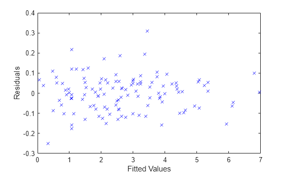
lme = fitlme(tbl,'y ~ InitialWeight + Program*Week + (Week|Subject)');

Compute the fitted values and raw residuals.

F = fitted(lme);
R = residuals(lme);

Plot the residuals versus the fitted values.

plot(F,R,'bx')
xlabel('Fitted Values')
ylabel('Residuals')

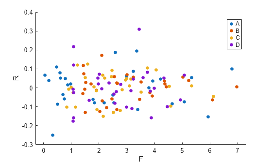
Now, plot the residuals versus the fitted values, grouped by program.

figure()
gscatter(F,R,Program)

Input Arguments

lme — Linear mixed-effects model

LinearMixedModel object

Linear mixed-effects model, specified as a LinearMixedModel object constructed using fitlme or fitlmematrix.

Name-Value Arguments

Specify optional pairs of arguments as Name1=Value1,...,NameN=ValueN, where Name is the argument name and Value is the corresponding value. Name-value arguments must appear after other arguments, but the order of the pairs does not matter.

Before R2021a, use commas to separate each name and value, and enclose Name in quotes.

Example: yfit = fitted(lme,'Conditional',false)

Conditional — Indicator for conditional response

true (default) | false

Indicator for conditional response, specified as the comma-separated pair consisting of 'Conditional' and either of the following.

true	Contribution from both fixed effects and random effects (conditional)
false	Contribution from only fixed effects (marginal)

Example: 'Conditional',false

Data Types: logical

Output Arguments

yfit — Fitted response values

n-by-1 vector

Fitted response values, returned as an n-by-1 vector, where n is the number of observations.

More About

Fitted Conditional and Marginal Response

A conditional response includes contributions from both fixed and random effects, whereas a marginal response includes contribution from only fixed effects.

Suppose the linear mixed-effects model, lme, has an n-by-p fixed-effects design matrix X and an n-by-q random-effects design matrix Z. Also, suppose the p-by-1 estimated fixed-effects vector is $$\widehat{\beta }$$, and the q-by-1 estimated best linear unbiased predictor (BLUP) vector of random effects is $$\widehat{b}$$. The fitted conditional response is

$${\widehat{y}}_{Cond}=X\widehat{\beta }+Z\widehat{b},$$

and the fitted marginal response is

$${\widehat{y}}_{Mar}=X\widehat{\beta },$$

Version History

Introduced in R2013b