Response Surface Demonstration Tool

Interactive response surface modeling demonstration

Description

The Response Surface Demonstration tool provides an interface for interactively investigating response surface methodology (RSM), nonlinear fitting, and the design of experiments.

The tool allows you to collect and model data from a simulated chemical reaction. The experimental predictors are the concentrations of three reactants (hydrogen, n-pentane, and isopentane) in pounds per square inch absolute units. The response variable (reaction rate) is simulated by a Hougen-Watson model (Bates and Watts, [1], pp. 271–272):

$$rate=\frac{{\beta }_1{X}_2-X_3/{\beta }_5}{1+{\beta }_2{X}_1+{\beta }_3{X}_2+{\beta }_4{X}_3}$$

where rate is the reaction rate; X₁, X₂, and X₃ are the concentrations of hydrogen, n-pentane, and isopentane, respectively; and β₁, β₂, ..., β₅ are fixed parameters. The software perturbs the reaction rate for each combination of reactant concentrations using random errors. You can set reactant concentration combinations manually, or use a set of combinations created using a D-optimal experiment design. For examples, see Manually Adjust Reactant Concentrations and Set Reactant Concentrations Using Experiment Design.

Required Products

• MATLAB^®

• Statistics and Machine Learning Toolbox™

Open the Response Surface Demonstration Tool

• At the MATLAB command prompt, enter rsmdemo.

Examples

Manually Adjust Reactant Concentrations

Use the Response Surface Demonstration tool to collect and model data from a simulated chemical reaction by manually adjusting the concentrations of three reactants.

In the Reaction Simulator window, adjust the reactant concentrations by editing the text boxes or dragging the associated sliders.

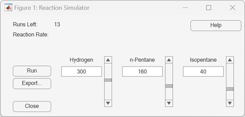
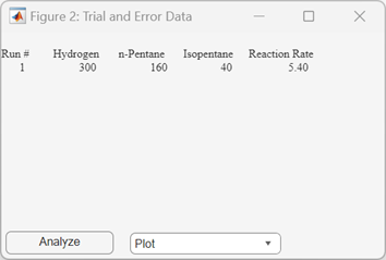
Click Run. The Trial and Error Data window displays the selected reactant concentrations and the simulated reaction rate for the first run..

To simulate another experiment run, adjust the reactant concentrations again, and then click Run. You can simulate up to 13 independent experimental runs for data collection. The Reaction Simulator window indicates the number of runs left.

After collecting at least 6 experimental runs, generate a scatter plot of the hydrogen concentration versus the reaction rate, with a line showing the fitted model. In the Trial and Error Data window, click Plot and select Hydrogen vs. Rate.

The solid line shows a linear regression model fit to the reaction rate as a function of the hydrogen concentration.

Fit a response surface model to the data by clicking Analyze in the Trial and Error Data window. The software loads the experiment data into the Response Surface Tool. By default, the tool fits the experiment data with a linear additive model. However, you can choose a different model using the menu at the bottom left of the rstool window.

Set Reactant Concentrations Using Experiment Design

Use the Response Surface Demonstration tool to collect and model data from a simulated chemical reaction according to an experiment design that sets reactant concentrations.

In the Experimental Data window, click Do Experiment.

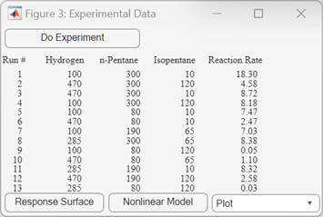
The software uses the cordexch function to generate a D-optimal design that sets the reactant concentrations for 13 runs. The Experimental Data window displays the concentrations and simulated reaction rates.

Fit a response surface model to the experiment data by clicking Response Surface in the Experimental Data window. The software loads the data into the Response Surface Tool. By default, the tool fits the experiment data with a full quadratic model. However, you can choose a different model using the menu at the bottom left of the rstool window.

Fit a Hougen-Watson model to the experiment data by clicking Nonlinear Model in the Experimental Data window. The software loads the data into the Nonlinear Regression Fitter Tool and fits it using hougen.

References

[1] Bates, D. M., and D. G. Watts. Nonlinear Regression Analysis and Its Applications. Hoboken, NJ: John Wiley & Sons, Inc., 1988.

Version History

Introduced before R2006a