Test Differences Between Category Means
This example shows how to test for significant differences between category (group) means using a t-test, two-way ANOVA (analysis of variance), and ANOCOVA (analysis of covariance) analysis.
Determine if the expected miles per gallon for a car depends on the decade in which it was manufactured or the location where it was manufactured.
Load Sample Data
load carsmall
unique(Model_Year)
ans = 3×1
70
76
82
The variable MPG has miles per gallon measurements on a sample of 100 cars. The variables Model_Year and Origin contain the model year and country of origin for each car.
The first factor of interest is the decade of manufacture. There are three manufacturing years in the data.
Create Factor for Decade of Manufacture
Create a categorical array named Decade by merging the observations from years 70 and 76 into a category labeled 1970s, and putting the observations from 82 into a category labeled 1980s.
Decade = discretize(Model_Year,[70 77 82], ...
    "categorical",["1970s","1980s"]);
categories(Decade)
ans = 2×1 cell
    {'1970s'}
    {'1980s'}
Plot Data Grouped by Category
Draw a box plot of miles per gallon, grouped by the decade of manufacture.
boxplot(MPG,Decade)
title("Miles per Gallon, Grouped by Decade of Manufacture")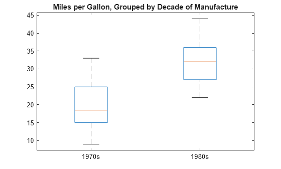
The box plot suggests that miles per gallon is higher in cars manufactured during the 1980s compared to the 1970s.
Compute Summary Statistics
Compute the mean and variance of miles per gallon for each decade.
[xbar,s2,grp] = grpstats(MPG,Decade,["mean","var","gname"])
xbar = 2×1

   19.7857
   31.7097
s2 = 2×1

   35.1429
   29.0796
grp = 2×1 cell
    {'1970s'}
    {'1980s'}
This output shows that the mean miles per gallon in the 1980s was approximately 31.71, compared to 19.79 in the 1970s. The variances in the two groups are similar.
Conduct Two-Sample t-Test for Equal Group Means
Conduct a two-sample t-test, assuming equal variances, to test for a significant difference between the group means. The hypothesis is
MPG70 = MPG(Decade=="1970s");
MPG80 = MPG(Decade=="1980s");
[h,p] = ttest2(MPG70,MPG80)
h =
1
p =
3.4809e-15
The logical value 1 indicates the null hypothesis is rejected at the default 0.05 significance level. The p-value for the test is very small. There is sufficient evidence that the mean miles per gallon in the 1980s differs from the mean miles per gallon in the 1970s.
Create Factor for Location of Manufacture
The second factor of interest is the location of manufacture. First, convert Origin to a categorical array.
Location = categorical(cellstr(Origin));
tabulate(Location)
    Value    Count   Percent
   France        4      4.00%
  Germany        9      9.00%
    Italy        1      1.00%
    Japan       15     15.00%
   Sweden        2      2.00%
      USA       69     69.00%
There are six different countries of manufacture. The European countries have relatively few observations.
Merge Categories
Combine the categories France, Germany, Italy, and Sweden into a new category named Europe.
Location = mergecats(Location, ...
    ["France","Germany","Italy","Sweden"],"Europe");
tabulate(Location)
   Value    Count   Percent
  Europe       16     16.00%
   Japan       15     15.00%
     USA       69     69.00%
Compute Summary Statistics
Compute the mean miles per gallon, grouped by the location of manufacture.
[meanMPG,locationGroup] = grpstats(MPG,Location,["mean","gname"])
meanMPG = 3×1

   26.6667
   31.8000
   21.1328
locationGroup = 3×1 cell
    {'Europe'}
    {'Japan' }
    {'USA'   }
This result shows that average miles per gallon is lowest for the sample of cars manufactured in the U.S.
Conduct Two-Way ANOVA
Conduct a two-way ANOVA to test for differences in expected miles per gallon between factor levels for Decade and Location.
The statistical model is
where is the response, miles per gallon, for cars made in decade at location . The treatment effects for the first factor, decade of manufacture, are the terms (constrained to sum to zero). The treatment effects for the second factor, location of manufacture, are the terms (constrained to sum to zero). The are uncorrelated, normally distributed noise terms.
The hypotheses to test are equality of decade effects,
and equality of location effects,
You can conduct a multiple-factor ANOVA using anovan.
anovan(MPG,{Decade,Location}, ...
    "Varnames",["Decade","Location"]);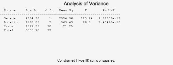
This output shows the results of the two-way ANOVA. The p-value for testing the equality of decade effects is 2.88503e-18, so the null hypothesis is rejected at the 0.05 significance level. The p-value for testing the equality of location effects is 7.40416e-10, so this null hypothesis is also rejected.
Conduct ANOCOVA Analysis
A potential confounder in this analysis is car weight. Cars with greater weight are expected to have lower gas mileage. Include the variable Weight as a continuous covariate in the ANOVA; that is, conduct an ANOCOVA analysis.
Assuming parallel lines, the statistical model is
The difference between this model and the two-way ANOVA model is the inclusion of the continuous predictor , the weight for the th car, which was made in the th decade and in theth location. The slope parameter is .
Add the continuous covariate as a third group in the second anovan input argument. Use the Continuous name-value argument to specify that Weight (the third group) is continuous.
anovan(MPG,{Decade,Location,Weight},"Continuous",3, ...
    "Varnames",["Decade","Location","Weight"]);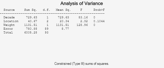
This output shows that when car weight is considered, there is insufficient evidence of a manufacturing location effect (p-value = 0.1044).
Use Interactive Tool
You can use the interactive aoctool to explore this result. This command opens three dialog boxes.
aoctool(Weight,MPG,Location);
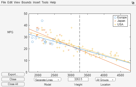


In the ANOCOVA Prediction Plot dialog box, select the Separate Means model.
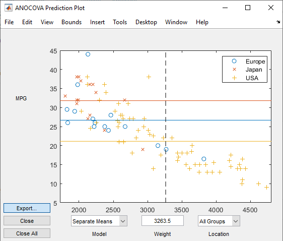
This output shows that when you do not include Weight in the model, there are fairly large differences in the expected miles per gallon among the three manufacturing locations. Note that here the model does not adjust for the decade of manufacturing.
Now, select the Parallel Lines model.
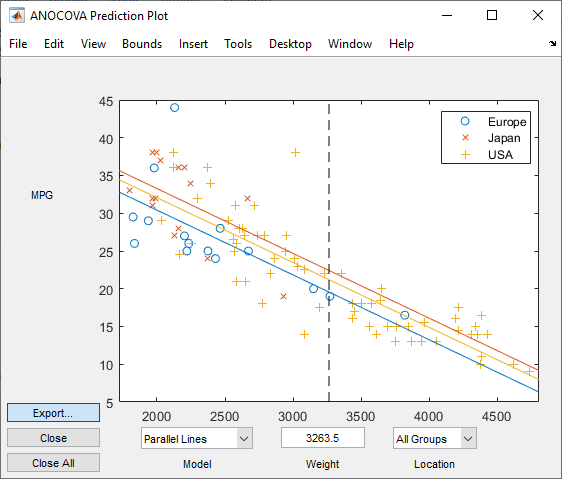
When you include Weight in the model, the difference in expected miles per gallon among the three manufacturing locations is much smaller.
See Also
categorical | boxplot | grpstats | ttest2 | anovan | aoctool