Main Content

dualtree3

3-D dual-tree complex wavelet transform

Description

[a,d] = dualtree3(x) returns the 3-D dual-tree complex wavelet transform of x at the maximum level, floor(log2(min(size(x)))).

[a,d] = dualtree3(x,level) returns the 3-D dual-tree wavelet transform down to level.

example

[a,d] = dualtree3(___,Name,Value) specifies options using name-value pair arguments in addition to any of the input arguments in previous syntaxes.

example

[a,d] = dualtree3(___,'excludeL1') excludes the first-level wavelet (detail) coefficients. Excluding the first-level wavelet coefficients can speed up the algorithm and saves memory. The first level does not exhibit the directional selectivity of levels 2 and higher. The perfect reconstruction property of the dual-tree wavelet transform holds only if the first-level wavelet coefficients are included. If you do not specify this option, or append 'includeL1', then the function includes the first-level coefficients.

Examples

collapse all

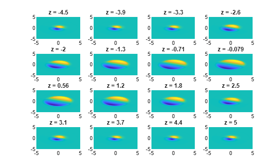
Generate a volumetric data set. Plot several cross-sections of the data seen from above. The data are not symmetric about the x-axis or the y-axis.

xl = 64;

xx = linspace(-5,5,xl);

[x,y,z] = meshgrid(xx);

G = (x+3*y)./(1+exp((x.^2+2*y.^2+z.^2)-10));

for k = 1:16
    subplot(4,4,k)
    surf(xx,xx,G(:,:,4*k))
    view(2)
    shading interp
    title(['z = ' num2str(xx(4*k),2)])
end

Figure contains 16 axes objects. Axes object 1 with title z = -4.5 contains an object of type surface. Axes object 2 with title z = -3.9 contains an object of type surface. Axes object 3 with title z = -3.3 contains an object of type surface. Axes object 4 with title z = -2.6 contains an object of type surface. Axes object 5 with title z = -2 contains an object of type surface. Axes object 6 with title z = -1.3 contains an object of type surface. Axes object 7 with title z = -0.71 contains an object of type surface. Axes object 8 with title z = -0.079 contains an object of type surface. Axes object 9 with title z = 0.56 contains an object of type surface. Axes object 10 with title z = 1.2 contains an object of type surface. Axes object 11 with title z = 1.8 contains an object of type surface. Axes object 12 with title z = 2.5 contains an object of type surface. Axes object 13 with title z = 3.1 contains an object of type surface. Axes object 14 with title z = 3.7 contains an object of type surface. Axes object 15 with title z = 4.4 contains an object of type surface. Axes object 16 with title z = 5 contains an object of type surface.

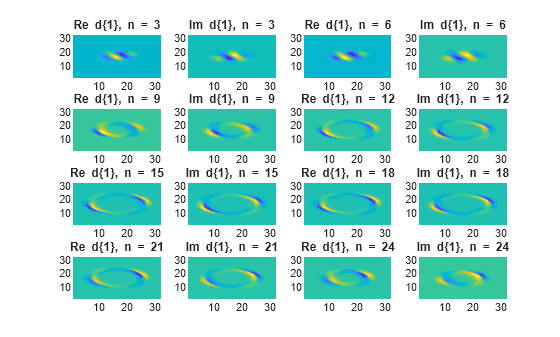
Compute the 3-D dual-tree transform of the data down to level 4. Specify a Hilbert Q-shift filter-pair length of 14.

[a,d] = dualtree3(G,4,'FilterLength',14);

Plot the real and imaginary parts of the first-level wavelet coefficients for selected subbands. The coefficients have the same directionality as the data. The imaginary parts are shifted versions of the real parts.

m = 1;

for k = 1:8
    subplot(4,4,2*k-1)
    surf(real(d{m}(:,:,3*k)))

    view(2)
    shading interp
    axis tight
    title(['Re d\{1\}, n = ' int2str(3*k)])

    subplot(4,4,2*k)
    surf(imag(d{m}(:,:,3*k)))

    view(2)
    shading interp
    axis tight
    title(['Im d\{1\}, n = ' int2str(3*k)])
end

Figure contains 16 axes objects. Axes object 1 with title Re d { 1 } , blank n blank = blank 3 contains an object of type surface. Axes object 2 with title Im d { 1 } , blank n blank = blank 3 contains an object of type surface. Axes object 3 with title Re d { 1 } , blank n blank = blank 6 contains an object of type surface. Axes object 4 with title Im d { 1 } , blank n blank = blank 6 contains an object of type surface. Axes object 5 with title Re d { 1 } , blank n blank = blank 9 contains an object of type surface. Axes object 6 with title Im d { 1 } , blank n blank = blank 9 contains an object of type surface. Axes object 7 with title Re d { 1 } , blank n blank = 12 contains an object of type surface. Axes object 8 with title Im d { 1 } , blank n blank = 12 contains an object of type surface. Axes object 9 with title Re d { 1 } , blank n blank = 15 contains an object of type surface. Axes object 10 with title Im d { 1 } , blank n blank = 15 contains an object of type surface. Axes object 11 with title Re d { 1 } , blank n blank = 18 contains an object of type surface. Axes object 12 with title Im d { 1 } , blank n blank = 18 contains an object of type surface. Axes object 13 with title Re d { 1 } , blank n blank = 21 contains an object of type surface. Axes object 14 with title Im d { 1 } , blank n blank = 21 contains an object of type surface. Axes object 15 with title Re d { 1 } , blank n blank = 24 contains an object of type surface. Axes object 16 with title Im d { 1 } , blank n blank = 24 contains an object of type surface.

Repeat the procedure for the second-level coefficients. When the level number increases by one, the array of wavelet coefficients decreases by half along the first two dimensions.

m = 2;

for k = 1:8
    subplot(4,4,2*k-1)
    surf(real(d{m}(:,:,3*k)))

    view(2)
    shading interp
    axis tight
    title(['Re d\{2\}, n = ' int2str(3*k)])

    subplot(4,4,2*k)
    surf(imag(d{m}(:,:,3*k)))

    view(2)
    shading interp
    axis tight
    title(['Im d\{2\}, n = ' int2str(3*k)])
end

Figure contains 16 axes objects. Axes object 1 with title Re d { 2 } , blank n blank = blank 3 contains an object of type surface. Axes object 2 with title Im d { 2 } , blank n blank = blank 3 contains an object of type surface. Axes object 3 with title Re d { 2 } , blank n blank = blank 6 contains an object of type surface. Axes object 4 with title Im d { 2 } , blank n blank = blank 6 contains an object of type surface. Axes object 5 with title Re d { 2 } , blank n blank = blank 9 contains an object of type surface. Axes object 6 with title Im d { 2 } , blank n blank = blank 9 contains an object of type surface. Axes object 7 with title Re d { 2 } , blank n blank = 12 contains an object of type surface. Axes object 8 with title Im d { 2 } , blank n blank = 12 contains an object of type surface. Axes object 9 with title Re d { 2 } , blank n blank = 15 contains an object of type surface. Axes object 10 with title Im d { 2 } , blank n blank = 15 contains an object of type surface. Axes object 11 with title Re d { 2 } , blank n blank = 18 contains an object of type surface. Axes object 12 with title Im d { 2 } , blank n blank = 18 contains an object of type surface. Axes object 13 with title Re d { 2 } , blank n blank = 21 contains an object of type surface. Axes object 14 with title Im d { 2 } , blank n blank = 21 contains an object of type surface. Axes object 15 with title Re d { 2 } , blank n blank = 24 contains an object of type surface. Axes object 16 with title Im d { 2 } , blank n blank = 24 contains an object of type surface.

Invert the transform, specifying the same filter-pair length. Check for perfect reconstruction.

xrec = idualtree3(a,d,'FilterLength',14);
max(abs(xrec(:)-G(:)))
ans = 1.9984e-14

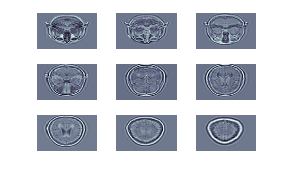
Load a set of MRI measurements of a human head. Truncate the data so that it is even along the third dimension. Compute the 3-D dual-tree transform, excluding the first-level wavelet coefficients.

load wmri

[A,D] = dualtree3(X(:,:,1:26),2,'excludeL1');

Reconstruct the data by inverting the transform. Set the final-level scaling coefficients explicitly to 0. Display an evenly spaced selection of reconstructed images.

imrec = idualtree3(A*0,D);

colormap bone
for kj = 1:9
    subplot(3,3,kj)
    surf(imrec(:,:,3*kj-2))
    shading interp
    view(2)
    axis tight off
end

Input Arguments

collapse all

Input data, specified as a real 3-D array. All three dimensions of x must be even and greater than or equal to 4.

Data Types: double | single

Transform level, specified as a positive integer greater than or equal to 2 and less than or equal to floor(log2(min(size(x)))).

Data Types: double | single

Name-Value Arguments

Specify optional pairs of arguments as Name1=Value1,...,NameN=ValueN, where Name is the argument name and Value is the corresponding value. Name-value arguments must appear after other arguments, but the order of the pairs does not matter.

Before R2021a, use commas to separate each name and value, and enclose Name in quotes.

Example: 'LevelOneFilter','legall','FilterLength',6 computes a transform using LeGall analysis filters with scaling length 5 and wavelet length 3 at level 1, and length-6 Q-shift filters at levels 2 and greater.

Hilbert Q-shift filter-pair length, specified as the comma-separated pair consisting of 'FilterLength' and one of 6, 10, 14, 16, or 18. dualtree3 uses the orthogonal Hilbert Q-shift filter pair of length 'FilterLength' for levels 2 and greater.

Data Types: double | single

First-level biorthogonal analysis filter, specified as the comma-separated pair consisting of 'LevelOneFilter' and a character vector or string. By default, dualtree3 uses for level 1 the near-symmetric biorthogonal wavelet filter with lengths 5 (scaling filter) and 7 (wavelet filter).

Data Types: char | string

Output Arguments

collapse all

Final-level scaling (lowpass) coefficients, returned as a real-valued matrix.

Data Types: double

Wavelet coefficients, returned as a 1-by-level cell array. There are 28 wavelet subbands in the 3-D dual-tree transform at each level.

Data Types: double
Complex Number Support: Yes

References

[1] Chen, H., and N. G. Kingsbury. “Efficient Registration of Nonrigid 3-D Bodies.” IEEE® Transactions on Image Processing. Vol 21, January 2012, pp. 262–272.

[2] Kingsbury, N. G. “Complex Wavelets for Shift Invariant Analysis and Filtering of Signals.” Journal of Applied and Computational Harmonic Analysis, Vol. 10, Number 3, May 2001, pp. 234–253.

Version History

Introduced in R2017a