Dual-Tree Complex Wavelet Transforms
This example shows how the dual-tree complex wavelet transform (DTCWT) provides advantages over the critically sampled DWT for signal, image, and volume processing. The DTCWT is implemented as two separate two-channel filter banks. To gain the advantages described in this example, you cannot arbitrarily choose the scaling and wavelet filters used in the two trees. The lowpass (scaling) and highpass (wavelet) filters of one tree, , must generate a scaling function and wavelet that are approximate Hilbert transforms of the scaling function and wavelet generated by the lowpass and highpass filters of the other tree, . Therefore, the complex-valued scaling functions and wavelets formed from the two trees are approximately analytic.
As a result, the DTCWT exhibits less shift variance and more directional selectivity than the critically sampled DWT with only a redundancy factor for -dimensional data. The redundancy in the DTCWT is significantly less than the redundancy in the undecimated (stationary) DWT.
This example illustrates the approximate shift invariance of the DTCWT, the selective orientation of the dual-tree analyzing wavelets in 2-D and 3-D, and the use of the dual-tree complex discrete wavelet transform in image and volume denoising.
Near Shift Invariance of the DTCWT
The DWT suffers from shift variance, meaning that small shifts in the input signal or image can cause significant changes in the distribution of signal/image energy across scales in the DWT coefficients. The DTCWT is approximately shift invariant.
To demonstrate this on a test signal, construct two shifted discrete-time impulses 128 samples in length. One signal has the unit impulse at sample 60, while the other signal has the unit impulse at sample 64. Both signals clearly have unit energy ( norm).
kronDelta1 = zeros(128,1);
kronDelta1(60) = 1;
kronDelta2 = zeros(128,1);
kronDelta2(64) = 1;
Set the DWT extension mode to periodic. Obtain the DWT and DTCWT of the two signals down to level 3 with wavelet and scaling filters of length 14. Extract the level-3 detail coefficients for comparison.
origmode = dwtmode('status','nodisplay');
dwtmode('per','nodisp')
J = 3;
[dwt1C,dwt1L] = wavedec(kronDelta1,J,'sym7');
[dwt2C,dwt2L] = wavedec(kronDelta2,J,'sym7');
dwt1Cfs = detcoef(dwt1C,dwt1L,3);
dwt2Cfs = detcoef(dwt2C,dwt2L,3);

[dt1A,dt1D] = dualtree(kronDelta1,'Level',J,'FilterLength',14);
[dt2A,dt2D] = dualtree(kronDelta2,'Level',J,'FilterLength',14);
dt1Cfs = dt1D{3};
dt2Cfs = dt2D{3};
Plot the absolute values of the DWT and DTCWT coefficients for the two signals at level 3 and compute the energy (squared norms) of the coefficients. Plot the coefficients on the same scale. The four sample shift in the signal has caused a significant change in the energy of the level-3 DWT coefficients. The energy in the level-3 DTCWT coefficients has changed by only approximately 3%.
figure
tiledlayout(1,2)
nexttile
stem(abs(dwt1Cfs),'markerfacecolor',[0 0 1])
title({'DWT';['Squared 2-norm = ' num2str(norm(dwt1Cfs,2)^2,3)]},...
    'fontsize',10)
ylim([0 0.4])
nexttile
stem(abs(dwt2Cfs),'markerfacecolor',[0 0 1])
title({'DWT';['Squared 2-norm = ' num2str(norm(dwt2Cfs,2)^2,3)]},...
    'fontsize',10)
ylim([0 0.4])
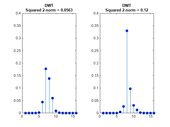
figure
tiledlayout(1,2)
nexttile
stem(abs(dt1Cfs),'markerfacecolor',[0 0 1])
title({'Dual-tree CWT';['Squared 2-norm = ' num2str(norm(dt1Cfs,2)^2,3)]},...
    'fontsize',10)
ylim([0 0.4])
nexttile
stem(abs(dwt2Cfs),'markerfacecolor',[0 0 1])
title({'Dual-tree CWT';['Squared 2-norm = ' num2str(norm(dt2Cfs,2)^2,3)]},...
    'fontsize',10)
ylim([0 0.4])

To demonstrate the utility of approximate shift invariance in real data, we analyze an electrocardiogram (ECG) signal. The sampling interval for the ECG signal is 1/180 seconds. The data are taken from Percival & Walden [3], p.125 (data originally provided by William Constantine and Per Reinhall, University of Washington). For convenience, we take the data to start at t=0.
load wecg
dt = 1/180;
t = 0:dt:(length(wecg)*dt)-dt;
figure
plot(t,wecg)
xlabel('Seconds')
ylabel('Millivolts')

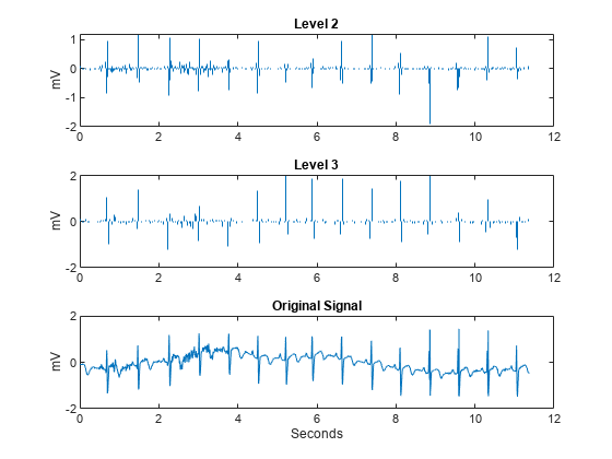
The large positive peaks approximately 0.7 seconds apart are the R waves of the cardiac rhythm. First, decompose the signal using the critically sampled DWT with the Farras nearly symmetric filters. Plot the original signal along with the level-2 and level-3 wavelet coefficients. The level-2 and level-3 coefficients were chosen because the R waves are isolated most prominently in those scales for the given sampling rate.
figure
J = 6;
[df,rf] = dtfilters('farras');
[dtDWT1,L1] = wavedec(wecg,J,df(:,1),df(:,2));
details = zeros(2048,3);
details(2:4:end,2) = detcoef(dtDWT1,L1,2);
details(4:8:end,3) = detcoef(dtDWT1,L1,3);
tiledlayout(3,1)
nexttile
stem(t,details(:,2),'Marker','none','ShowBaseline','off')
title('Level 2')
ylabel('mV')
nexttile
stem(t,details(:,3),'Marker','none','ShowBaseline','off')
title('Level 3')
ylabel('mV')
nexttile
plot(t,wecg)
title('Original Signal')
xlabel('Seconds')
ylabel('mV')
Repeat the above analysis for the dual-tree transform. In this case, just plot the real part of the dual-tree coefficients at levels 2 and 3.
[dtcplxA,dtcplxD] = dualtree(wecg,'Level',J,'FilterLength',14);
details = zeros(2048,3);
details(2:4:end,2) = dtcplxD{2};
details(4:8:end,3) = dtcplxD{3};
tiledlayout(3,1)
nexttile
stem(t,real(details(:,2)),'Marker','none','ShowBaseline','off')
title('Level 2')
ylabel('mV')
nexttile
stem(t,real(details(:,3)),'Marker','none','ShowBaseline','off')
title('Level 3')
ylabel('mV')
nexttile
plot(t,wecg)
title('Original Signal')
xlabel('Seconds')
ylabel('mV')

Both the critically sampled and dual-tree wavelet transforms localize an important feature of the ECG waveform to similar scales
An important application of wavelets in 1-D signals is to obtain an analysis of variance by scale. It stands to reason that this analysis of variance should not be sensitive to circular shifts in the input signal. Unfortunately, this is not the case with the critically sampled DWT. To demonstrate this, we circularly shift the ECG signal by 4 samples, analyze the unshifted and shifted signals with the critically sampled DWT, and calculate the distribution of energy across scales.
wecgShift = circshift(wecg,4);
[dtDWT2,L2] = wavedec(wecgShift,J,df(:,1),df(:,2));

detCfs1 = detcoef(dtDWT1,L1,1:J,'cells');
apxCfs1 = appcoef(dtDWT1,L1,rf(:,1),rf(:,2),J);
cfs1 = horzcat(detCfs1,{apxCfs1});
detCfs2 = detcoef(dtDWT2,L2,1:J,'cells');
apxCfs2 = appcoef(dtDWT2,L2,rf(:,1),rf(:,2),J);
cfs2 = horzcat(detCfs2,{apxCfs2});

sigenrgy = norm(wecg,2)^2;
enr1 = cell2mat(cellfun(@(x)(norm(x,2)^2/sigenrgy)*100,cfs1,'uni',0));
enr2 = cell2mat(cellfun(@(x)(norm(x,2)^2/sigenrgy)*100,cfs2,'uni',0));
levels = {'D1';'D2';'D3';'D4';'D5';'D6';'A6'};
enr1 = enr1(:);
enr2 = enr2(:);
table(levels,enr1,enr2,'VariableNames',{'Level','enr1','enr2'})
ans=7×3 table
    Level      enr1      enr2
    ______    ______    ______

    {'D1'}    4.1994    4.1994
    {'D2'}     8.425     8.425
    {'D3'}    13.381    10.077
    {'D4'}    7.0612    10.031
    {'D5'}    5.4606    5.4436
    {'D6'}    3.1273    3.4584
    {'A6'}    58.345    58.366
Note that the wavelet coefficients at levels 3 and 4 show approximately 3% changes in energy between the original and shifted signal. Next, we repeat this analysis using the complex dual-tree discrete wavelet transform.
[dtcplx2A,dtcplx2D] = dualtree(wecgShift,'Level',J,'FilterLength',14);
dtCfs1 = vertcat(dtcplxD,{dtcplxA});
dtCfs2 = vertcat(dtcplx2D,{dtcplx2A});

dtenr1 = cell2mat(cellfun(@(x)(norm(x,2)^2/sigenrgy)*100,dtCfs1,'uni',0));
dtenr2 = cell2mat(cellfun(@(x)(norm(x,2)^2/sigenrgy)*100,dtCfs2,'uni',0));
dtenr1 = dtenr1(:);
dtenr2 = dtenr2(:);
table(levels,dtenr1,dtenr2, 'VariableNames',{'Level','dtenr1','dtenr2'})
ans=7×3 table
    Level     dtenr1    dtenr2
    ______    ______    ______

    {'D1'}    5.3533    5.3619
    {'D2'}    6.2672    6.2763
    {'D3'}    12.155     12.19
    {'D4'}    8.2831     8.325
    {'D5'}      5.81    5.8577
    {'D6'}    3.1768    3.0526
    {'A6'}    58.403    58.384
The dual-tree transform produces a consistent analysis of variance by scale for the original signal and its circularly shifted version.
Directional Selectivity in Image Processing
The standard implementation of the DWT in 2-D uses separable filtering of the columns and rows of the image. Use the helper function helperPlotCritSampDWT to plot the LH, HL, and HH wavelets for Daubechies' least-asymmetric phase wavelet with 4 vanishing moments, sym4.
helperPlotCritSampDWT

Note that the LH and HL wavelets have clear horizontal and vertical orientations respectively. However, the HH wavelet on the far right mixes both the +45 and -45 degree directions, producing a checkerboard artifact. This mixing of orientations is due to the use of real-valued separable filters. The HH real-valued separable filter has passbands in all four high frequency corners of the 2-D frequency plane.
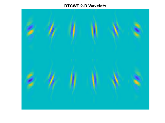
The dual-tree DWT achieves directional selectivity by using wavelets that are approximately analytic, meaning that they have support on only one half of the frequency axis. In the dual-tree DWT, there are six subbands for both the real and imaginary parts. The six real parts are formed by adding the outputs of column filtering followed by row filtering of the input image in the two trees. The six imaginary parts are formed by subtracting the outputs of column filtering followed by row filtering.
The filters applied to the columns and rows may be from the same filter pair, or , or from different filter pairs, . Use the helper function helperPlotWaveletDTCWT to plot the orientation of the 12 wavelets corresponding to the real and imaginary parts of the DTCWT. The top row of the preceding figure shows the real parts of the six wavelets, and the second row shows the imaginary parts.
helperPlotWaveletDTCWT
Edge Representation in Two Dimensions
The approximate analyticity and selective orientation of the complex dual-tree wavelets provide superior performance over the standard 2-D DWT in the representation of edges in images. To illustrate this, we analyze test images with edges consisting of line and curve singularities in multiple directions using the critically sampled 2-D DWT and the 2-D complex oriented dual-tree transform. First, analyze an image of an octagon, which consists of line singularities.
load woctagon
imagesc(woctagon)
colormap gray
title('Original Image')
axis equal
axis off

Use the helper function helperPlotOctagon to decompose the image down to level 4 and reconstruct an image approximation based on the level-4 detail coefficients.
helperPlotOctagon(woctagon)

Next, analyze an octagon with hyperbolic edges. The edges in the hyperbolic octagon are curve singularities.
load woctagonHyperbolic
figure
imagesc(woctagonHyperbolic)
colormap gray
title('Octagon with Hyperbolic Edges')
axis equal
axis off

Again, use the helper function helperPlotOctagon to decompose the image down to level 4 and reconstruct an image approximation based on the level-4 detail coefficients for both the standard 2-D DWT and the complex oriented dual-tree DWT.
helperPlotOctagon(woctagonHyperbolic)

Note that the ringing artifacts evident in the 2-D critically sampled DWT are absent in the 2-D DTCWT of both images. The DTCWT more faithfully reproduces line and curve singularities.
Image Denoising
Because of the ability to isolate distinct orientations in separate subbands, the DTCWT is often able to outperform the standard separable DWT in applications like image denoising. To demonstrate this, use the helper function helperCompare2DDenoisingDTCWT. The helper function loads an image and adds zero-mean white Gaussian noise with . For a user-supplied range of thresholds, the function compares denoising using soft thresholding for the critically sampled DWT, and the DTCWT. For each threshold value, the root-mean-square (RMS) error and peak signal-to-noise ratio (PSNR) are displayed.
numex = 3;
helperCompare2DDenoisingDTCWT(numex,0:2:100,'PlotMetrics');
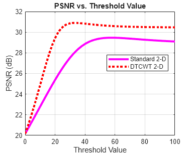
The DTCWT outperforms the standard DWT in RMS error and PSNR.
Next, obtain the denoised images for a threshold value of 25, which is equal to the standard deviation of the additive noise.
numex = 3;
helperCompare2DDenoisingDTCWT(numex,25,'PlotImage');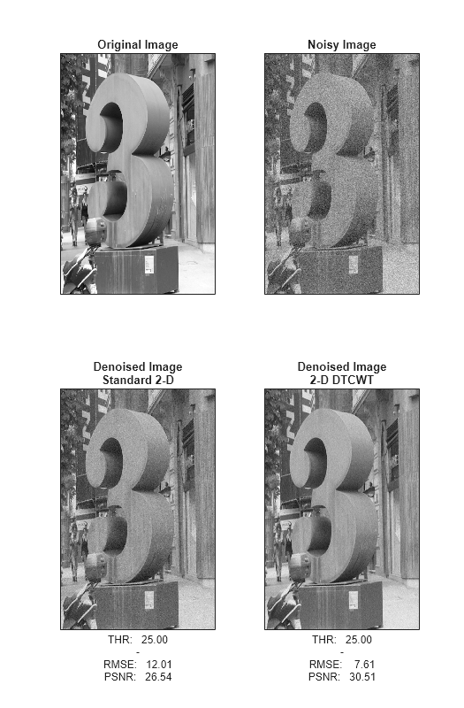
With a threshold value equal to the standard deviation of the additive noise, the DTCWT provides a PSNR almost 4 dB higher than the standard 2-D DWT.
Directional Selectivity in 3-D
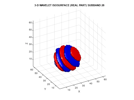
The ringing artifacts observed with the separable DWT in two dimensions is exacerbated when extending wavelet analysis to higher dimensions. The DTCWT enables you to maintain directional selectivity in 3-D with minimal redundancy. In 3-D, there are 28 wavelet subbands in the dual-tree transform.
To demonstrate the directional selectivity of the 3-D dual-tree wavelet transform, visualize example 3-D isosurfaces of both 3-D dual-tree and separable DWT wavelets. First, visualize the real and imaginary parts separately of two dual-tree subbands.
helperVisualize3D('Dual-Tree',28,'separate')

helperVisualize3D('Dual-Tree',25,'separate')


The red portion of the isosurface plot indicates the positive excursion of the wavelet from zero, while blue denotes the negative excursion. You can clearly see the directional selectivity in space of the real and imaginary parts of the dual-tree wavelets. Now visualize one of the dual-tree subbands with the real and imaginary plots plotted together as one isosurface.
helperVisualize3D('Dual-Tree',25,'real-imaginary')
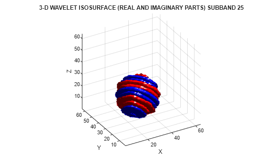
The preceding plot demonstrates that the real and imaginary parts are shifted versions of each other in space. This reflects the fact that the imaginary part of the complex wavelet is the approximate Hilbert transform of the real part. Next, visualize the isosurface of a real orthogonal wavelet in 3-D for comparison.
helperVisualize3D('DWT',7)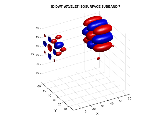
The mixing of orientations observed in the 2-D DWT is even more pronounced in 3-D. Just as in the 2-D case, the mixing of orientations in 3-D leads to significant ringing, or blocking artifacts. To demonstrate this, examine the 3-D DWT and DTCWT wavelet details of a spherical volume. The sphere is 64-by-64-by-64.
load sphr
[A,D] = dualtree3(sphr,2,'excludeL1');
A = zeros(size(A));
sphrDTCWT = idualtree3(A,D);
I = imtile(rescale(reshape(sphrDTCWT,[64 64 1 64])),GridSize=[8 8]);
imshow(I)
title('DTCWT Level 2 Details')
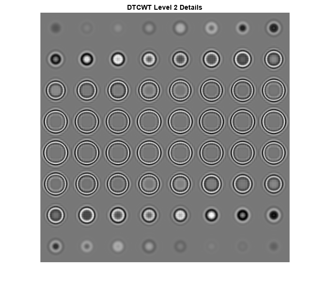
Compare the preceding plot against the second-level details based on the separable DWT.
sphrDEC = wavedec3(sphr,2,'sym4','mode','per');
sphrDEC.dec{1} = zeros(size(sphrDEC.dec{1}));
for kk = 2:8
    sphrDEC.dec{kk} = zeros(size(sphrDEC.dec{kk}));
end
sphrrecDWT = waverec3(sphrDEC);
figure
I = imtile(rescale(reshape(sphrrecDWT,[64 64 1 64])),GridSize=[8 8]);
imshow(I)
title('DWT Level 2 Details')

Zoom in on the images in both the DTCWT and DWT montages and you will see how prominent the blocking artifacts in the DWT details are compared to the DTCWT.
Volume Denoising
Similar to the 2-D case, the directional selectivity of the 3-D DTCWT often leads to improvements in volume denoising.
To demonstrate this, consider an MRI data set consisting of 16 slices. Gaussian noise with a standard deviation of 10 has been added to the original data set. Display the noisy data set.
load MRI3D
I = imtile(rescale(reshape(noisyMRI,[128 128 1 16])),GridSize=[4 4]);
imshow(I)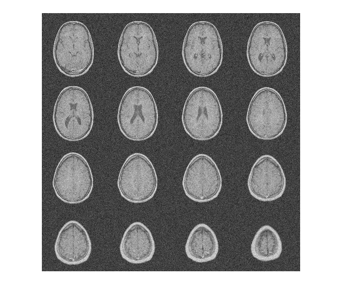
Note that the original SNR prior to denoising is approximately 11 dB.
20*log10(norm(origMRI(:),2)/norm(origMRI(:)-noisyMRI(:),2))
ans =
11.2997
Denoise the MRI dataset down to level 4 using both the DTCWT and the DWT. Similar wavelet filter lengths are used in both cases. Plot the resulting SNR as a function of the threshold. Display the denoised results for both the DTCWT and DWT obtained at the best SNR.
[imrecDTCWT,imrecDWT] = helperCompare3DDenoising(origMRI,noisyMRI);

figure
I = imtile(rescale(reshape(imrecDTCWT,[128 128 1 16])),GridSize=[4 4]);
imshow(I)
title('DTCWT Denoised Volume')
figure
I = imtile(rescale(reshape(imrecDWT,[128 128 1 16])),GridSize=[4 4]);
imshow(I)
title('DWT Denoised Volume')
Restore the original extension mode.
dwtmode(origmode,'nodisplay')Summary
We have shown that the dual-tree CWT possesses the desirable properties of near shift invariance and directional selectivity not achievable with the critically sampled DWT. We have demonstrated how these properties can result in improved performance in signal analysis, the representation of edges in images and volumes, and image and volume denoising.
References
Huizhong Chen, and N. Kingsbury. “Efficient Registration of Nonrigid 3-D Bodies.” IEEE Transactions on Image Processing 21, no. 1 (January 2012): 262–72. https://doi.org/10.1109/TIP.2011.2160958.
Kingsbury, Nick. “Complex Wavelets for Shift Invariant Analysis and Filtering of Signals.” Applied and Computational Harmonic Analysis 10, no. 3 (May 2001): 234–53. https://doi.org/10.1006/acha.2000.0343.
Percival, Donald B., and Andrew T. Walden. Wavelet Methods for Time Series Analysis. Cambridge Series in Statistical and Probabilistic Mathematics. Cambridge ; New York: Cambridge University Press, 2000.
Selesnick, I.W., R.G. Baraniuk, and N.C. Kingsbury. “The Dual-Tree Complex Wavelet Transform.” IEEE Signal Processing Magazine 22, no. 6 (November 2005): 123–51. https://doi.org/10.1109/MSP.2005.1550194.
Selesnick, I. "The Double Density DWT." Wavelets in Signal and Image Analysis: From Theory to Practice (A. A. Petrosian, and F. G. Meyer, eds.). Norwell, MA: Kluwer Academic Publishers, 2001, pp. 39–66.
Selesnick, I.W. “The Double-Density Dual-Tree DWT.” IEEE Transactions on Signal Processing 52, no. 5 (May 2004): 1304–14. https://doi.org/10.1109/TSP.2004.826174.
See Also
dualtree | dualtree2 | dualtree3