Main Content

dualtree2

Kingsbury Q-shift 2-D dual-tree complex wavelet transform

Since R2020a

Description

[A,D] = dualtree2(X) returns the 2-D dual-tree complex wavelet transform (DTCWT) of X using Kingsbury Q-shift filters. The output A is the matrix of real-valued final-level scaling (lowpass) coefficients. The output D is a L-by-1 cell array of complex-valued wavelet coefficients, where L is the level of the transform. For each element of D there are six wavelet subbands.

The DTCWT is obtained by default down to level floor(log2(min([H W]))), where H and W refer to the height (row dimension) and width (column dimension) of X, respectively. If any of the row or column dimensions of X are odd, X is extended along that dimension by reflecting around the last row or column.

By default, dualtree2 uses the near-symmetric biorthogonal wavelet filter pair with lengths 5 (scaling filter) and 7 (wavelet filter) for level 1 and the orthogonal Q-shift Hilbert wavelet filter pair of length 10 for levels greater than or equal to 2.

[___,Ascale] = dualtree2(X) returns the scaling (lowpass) coefficients at each level.

example

[___] = dualtree2(X,Name,Value) specifies additional options using name-value pair arguments. For example, 'LevelOneFilter','antonini' specifies the (9,7)-tap Antonini filter as the biorthogonal filter to use in the first-level analysis.

Examples

collapse all

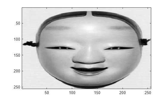
Load a grayscale image.

load mask
imagesc(X)
colormap gray

Figure contains an axes object. The axes object contains an object of type image.

Obtain the dual-tree complex wavelet transform of the image down to four levels of resolution.

[a,d] = dualtree2(X,'Level',4);

Display the final-level scaling (lowpass) coefficients.

imagesc(a)
colormap gray

Figure contains an axes object. The axes object contains an object of type image.

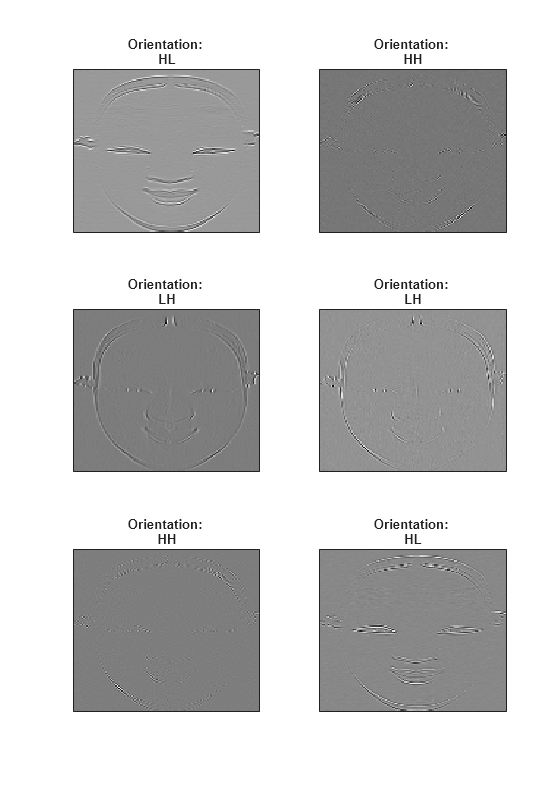
Display the tree B wavelet coefficients at the finest scale. Each subplot title denotes the particular subband ("H" for highpass, "L" for lowpass).

orientation = ["HL","HH","LH","LH","HH","HL"];
for k=1:6
    subplot(3,2,k)
    imagesc(imag(d{1}(:,:,k)))
    title(['Orientation: ' orientation(k)])
    set(gca,'xtick',[])
    set(gca,'ytick',[])
end
colormap gray
set(gcf,'Position',[0 0 560 800])

Figure contains 6 axes objects. Axes object 1 with title Orientation: HL contains an object of type image. Axes object 2 with title Orientation: HH contains an object of type image. Axes object 3 with title Orientation: LH contains an object of type image. Axes object 4 with title Orientation: LH contains an object of type image. Axes object 5 with title Orientation: HH contains an object of type image. Axes object 6 with title Orientation: HL contains an object of type image.

Input Arguments

collapse all

Input data, specified as a real-valued matrix, 3-D array, or 4-D array. X is a real-valued H-by-W-by-C-by-N array, where H is the height or row dimension, W is the width or column dimension, C is the number of channels, and N is the number of images. X must have at least two samples in each of the row and column dimensions.

Example: If X is a 256-by-256-by-3-by-2 array, X contains two 256-by-256 RGB images.

Data Types: double | single

Name-Value Arguments

Specify optional pairs of arguments as Name1=Value1,...,NameN=ValueN, where Name is the argument name and Value is the corresponding value. Name-value arguments must appear after other arguments, but the order of the pairs does not matter.

Before R2021a, use commas to separate each name and value, and enclose Name in quotes.

Example: 'LevelOneFilter','antonini','Level',4

Level of decomposition, specified as a positive integer less than or equal to floor(log2(min([H W]))), where H and W refer to the height (row dimension) and width (column dimension) of X, respectively. If unspecified, Level defaults to floor(log2(min([H W]))).

Biorthogonal filter to use in the first-level analysis, specified as:

  • 'legall' — LeGall 5/3 filter [3]

  • 'nearsym13_19' — (13,19)-tap near-orthogonal filter [2]

  • 'nearsym5_7' — (5,7)-tap near-orthogonal filter [1]

  • 'antonini' — (9,7)-tap Antonini filter [1]

By default, dualtree2 uses 'nearsym5_7', the near-symmetric biorthogonal filter pair with lengths 5 (scaling filter) and 7 (wavelet filter).

Orthogonal Hilbert Q-shift analysis filter pair length to use for levels 2 and higher, specified as one of the listed values [2]. By default, dualtree2 uses the orthogonal Q-shift Hilbert wavelet filter pair of length 10.

Output Arguments

collapse all

Final-level approximation coefficients, returned as a real-valued matrix.

Wavelet coefficients, returned as an L-by-1 cell array of complex-valued wavelet coefficients, where L is the level of the transform. The real parts of the coefficients are from tree A, and the imaginary parts are from tree B. For each element of D there are six wavelet subbands.

Approximation coefficients at each level of the transform, returned as an L-by-1 cell array of real-valued scaling (lowpass) coefficients, where L is the level of the transform. If X is a matrix, each element of D is a matrix whose column dimension equals the column dimension of X.

References

[1] Antonini, M., M. Barlaud, P. Mathieu, and I. Daubechies. “Image Coding Using Wavelet Transform.” IEEE Transactions on Image Processing 1, no. 2 (April 1992): 205–20. https://doi.org/10.1109/83.136597.

[2] Kingsbury, Nick. “Complex Wavelets for Shift Invariant Analysis and Filtering of Signals.” Applied and Computational Harmonic Analysis 10, no. 3 (May 2001): 234–53. https://doi.org/10.1006/acha.2000.0343.

[3] Le Gall, D., and A. Tabatabai. “Sub-Band Coding of Digital Images Using Symmetric Short Kernel Filters and Arithmetic Coding Techniques.” In ICASSP-88., International Conference on Acoustics, Speech, and Signal Processing, 761–64. New York, NY, USA: IEEE, 1988. https://doi.org/10.1109/ICASSP.1988.196696.

Extended Capabilities

C/C++ Code Generation
Generate C and C++ code using MATLAB® Coder™.

Version History

Introduced in R2020a